Receivers to Combat ISI and Their Analysis

4.4 Receivers to Combat ISI and Their Analysis

Section 4.3 assumed AWGN, which is a relatively simple channel that allows the transmitted signal to arrive at the receiver without distortion, with the added noise being the only impairment.

Here, the goal is to briefly study the effects of sending a signal through a frequency-selective channel (or, equivalently, a dispersive channel when considering the time domain), such as e. g. the $h_{c} (t)$ composing the LTI Gaussian channel of Eq. (4.1). Dispersive channels modify their input signals with respect to energy, spectrum, etc. To achieve a good performance in digital communication it is necessary to understand the effects of a frequency-selective channel and mitigate them.

With respect to the performance analysis of transmission systems in the presence of ISI, one strategy is to find an equivalent AWGN model. This allows the analysis to use concepts such as optimal matched filtering and deal with the effect of ISI as if it was non-white noise.

4.4.1 Intersymbol interference (ISI)

With a dispersive channel impulse response $h_{c} (t)≠δ(t)$ , one filtered symbol at the receiver can have a duration that exceeds its own interval of duration $T_{sym}$ and extend to the time interval of neighbors symbols. This is called intersymbol interference (ISI). For example, the impulse response of an average plain old telephony system (POTS) channel has a duration of approximately 10 ms. In this case, if one uses $R_{sym} = 2500$ bauds ( $T_{sym} = 0.4$ ms), a single symbol will influence approximately 25 neighboring symbols (i. e. the ISI will extend over approximately 25 symbols).

For example, assume a PAM with pulses of 100% duty cycle as in Figure 2.5. In this case, at the transmitter, a pulse corresponding to a new symbol begins just after the end of the pulse corresponding to the previous symbol. But the band limited channel can alter this harmony as indicated in Figure 2.6.

4.4.2 Pulse response

A channel that creates ISI is conveniently modeled by its overall pulse response. In the sequel, PAM is assumed for simplicity, but all development is valid for QAM (in this case the signals would be complex-valued) and even higher dimensions.

Note that extending the PAM generation of Block (2.15) to include the channel and receiver leads to the so-called ISI-channel model:

m[n]→ D/C → m_{s} (t)→ p_{t(t) →s(t)→ h_{c(t)} →r(t)→ p_{r(t)} →y(t).}

(4.17)

The shaping pulse at the transmitter is denoted here as $p_{t} (t)$ . Also for simplicity, it is assumed that $p_{t} (t)$ incorporates the impulse response of the transmitter filter $h_{Tx} (t)$ used e. g. in Eq. (2.2). Similarly, the receiver system impulse response $p_{r} (t)$ models all filtering processes that take place at the receiver.

Block (4.17) indicates that achieving zero ISI when dealing with $y(t)$ imposes requirements on the overall pulse response

p(t) = p_{t} (t)∗ h_{c} (t),

(4.18)

which is also called simply pulse response and corresponds to the cascade of all LTI systems used for modeling the complete chain composed of transmitter and channel⁶

Using Eq. (4.18), Block (4.17) can be depicted as:

m[n]→ D/C → m_{s} (t)→ p(t) →r(t).

(4.19)

From Block (4.19) and ignoring the receiver LTI $p_{r} (t)$ , given that $m_{s} (t) = ∑_{n=−∞}^{∞} m[n]δ(t − n T_{sym})$ , zero ISI is achieved when $r(n T_{sym}) = m[n]$ . In words, if there is no ISI, when sampling $r(t)$ for the $n$ -th symbol $m[n]$ , this sample $r(n T_{sym})$ depends only on $m[n]$ . Any signal $p(t)$ that leads to this situation is known as a zero-ISI Nyquist pulse.

The pulse response energy $E_{p}$ is an important parameter when studying the ISI impact

E_{p} = ||p(t)| |^{2} = < p(t),p(t) > = ∫_{−∞}^{∞} p(t) p^{∗} (t)dt.

(4.20)

In the sequel, examples of overall pulses $p(t)$ and the associated ISI are discussed in the context of PAM.

4.4.3 Examples of intersymbol interference (ISI) in PAM

The following three examples illustrate how $p(t)$ impacts a PAM signal, eventually creating ISI.

Example 4.6. Example of continuous-time Nyquist pulse shorter than $T_{sym}$ .

Figure 4.17: Example of achieving zero ISI by using a pulse $p(t)$ shorter than the symbol duration $T_{sym}$ . Figure 4.17(b) is a zoomed version of the middle graphic in Figure 4.17(a).

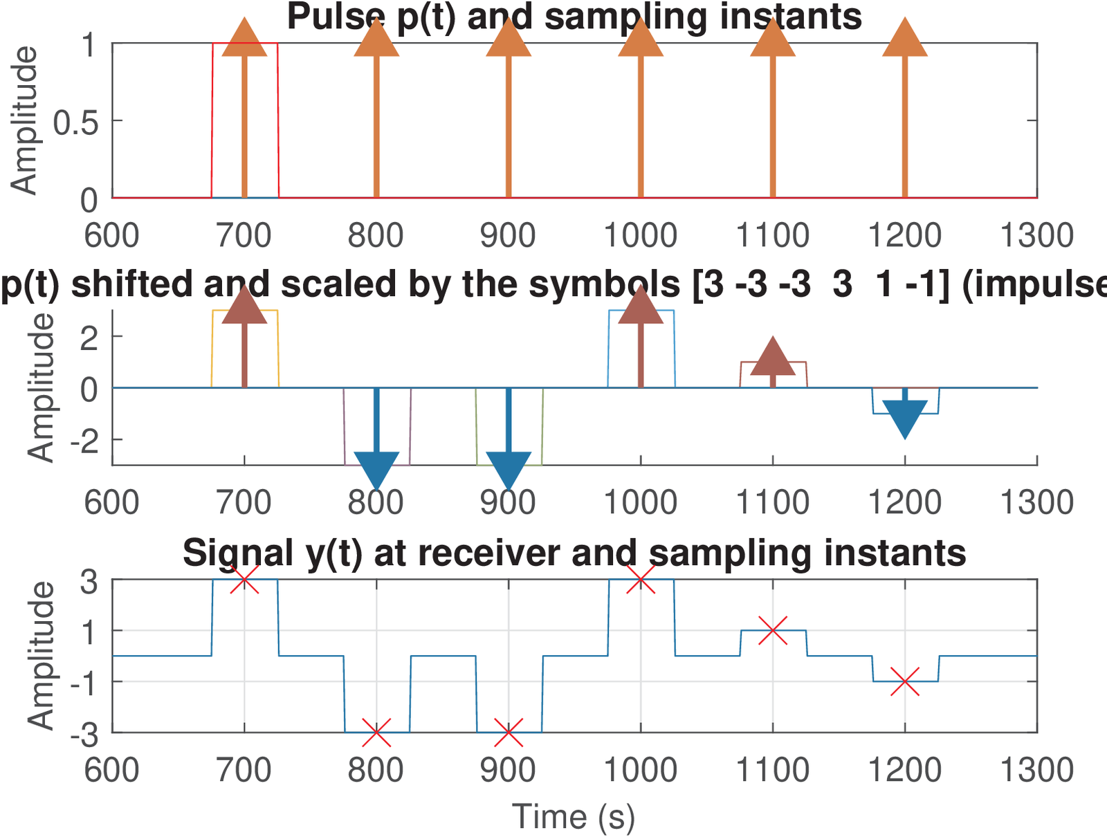
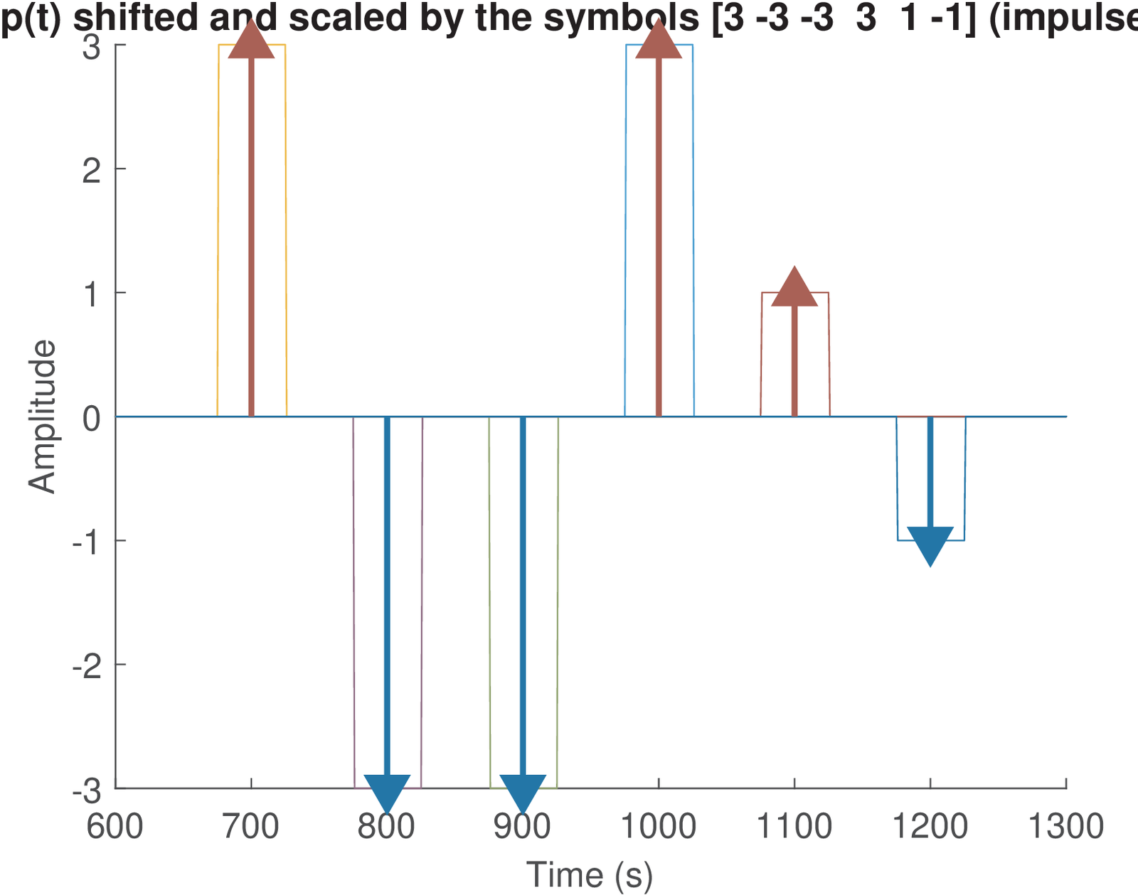
Figure 4.17 suggests a first solution to avoid ISI: constrain the duration of $p(t)$ to be shorter than the symbol duration $T_{sym}$ . The drawback of this strategy is that the shorter the pulse, the larger its BW, as suggested by Eq. (A.50). $□$

Example 4.7. Example of continuous-time Nyquist pulse longer than $T_{sym}$ .

Figure 4.18: Example of achieving zero ISI by using a Nyquist pulse $p(t)$ .

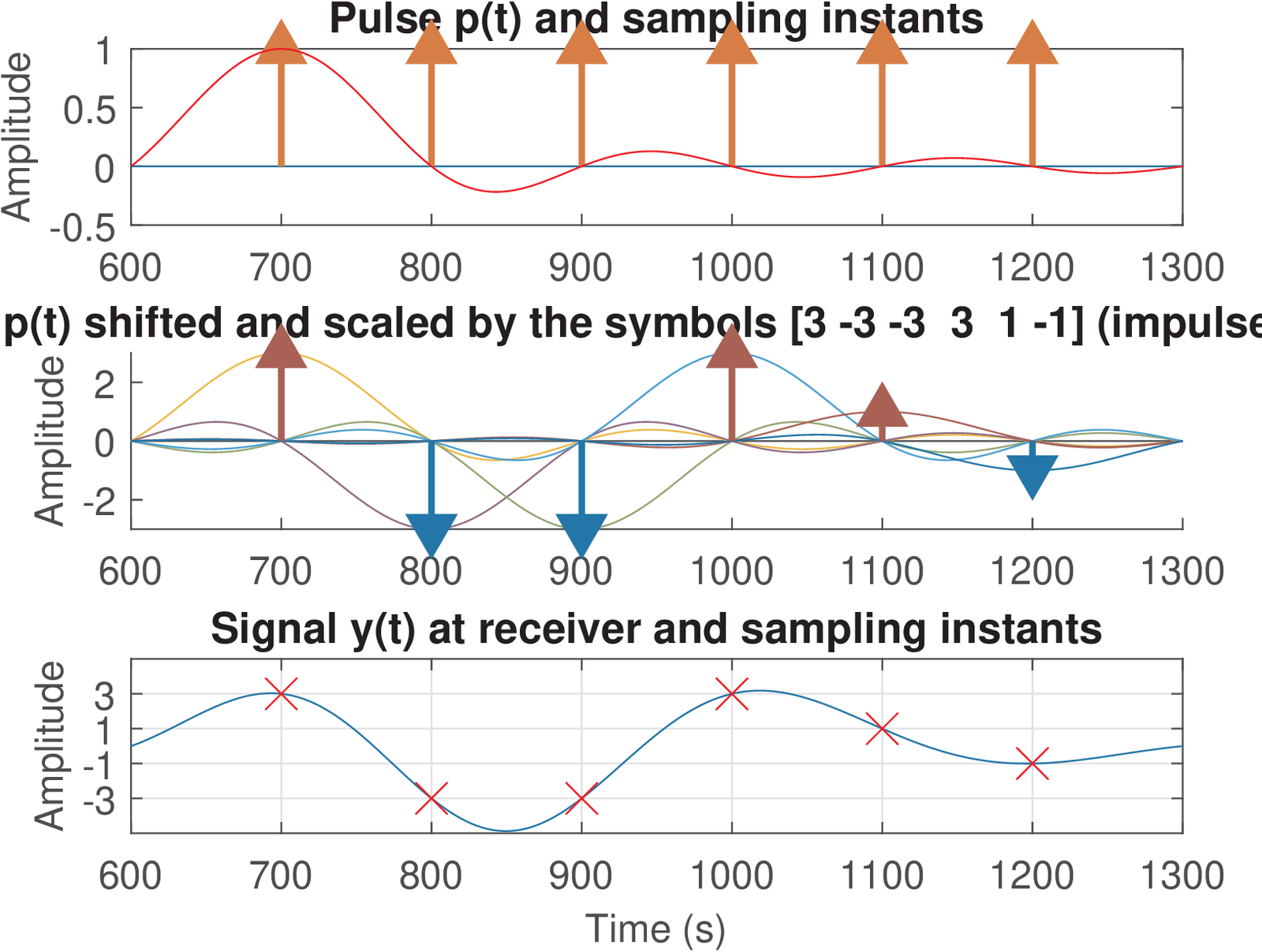
Figure 4.18 illustrates that a properly chosen pulse can achieve zero ISI: the amplitude of the pulse simply has to be zero at time instants $t = n T_{sym},n≠0$ . This is the distinctive property of a Nyquist pulse. When compared with Figure 4.17, the Nyquist pulse illustrated in Figure 4.18 can have its bandwidth reduced by using a pulse with support longer than $T_{sym}$ . $□$

Example 4.8. Example of continuous-time non-Nyquist pulse.

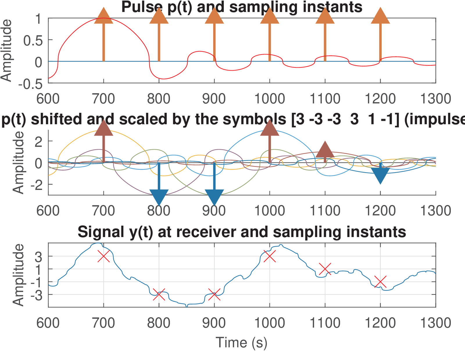
Figure 4.19: Example for which the ISI is non-zero because $p(t)$ is not a Nyquist pulse.

In contrast to Figure 4.17 and Figure 4.18, Figure 4.19 illustrates the consequence of using a pulse with support longer than $T_{sym}$ and that is not a Nyquist pulse. In this case, taking in account only the power at the sampling instants (the “ISI power”), one calculates 0.834 Watts for the specified samples. The power from this interference would add to the power of the background noise in case they are not correlated. $□$

4.4.4 Some practical aspects concerning the “pulse” to study ISI

The section discusses a model⁷ to study the performance of a communication system that faces ISI. First, some aspects of practical interest are discussed.

The overall pulse $p(t)$ determines the ISI of a system but, as indicated in Eq. (4.18), it has the inconvenience of depending on the channel $h_{c} (t)$ , which is not under control of the communication system designer. This can be circumvented by assuming that the channel was equalized and the combined effect of channel and equalizer is an ideal lowpass filter $h_{c} (t)$ . Besides, the spectrum $P_{t} (f) = F{p_{t} (t)}$ has to be assumed confined within the channel bandwidth $BW$ .⁸ Under these two assumptions, $h_{c} (t)$ does not distort the band-limited $s(t)$ and, consequently, $r(t) = s(t)$ in Block (4.17). This way one gets rid of the channel $h_{c} (t)$ in the model but should remember that the assumption is valid only if the transmitted signal is contained within the channel bandwidth, i. e., $P_{t} (f) ≈ 0$ for $f > BW$ .

With $h_{c} (t)$ eliminated, the pulse response Eq. (4.18) $p(t) = p_{t} (t)$ becomes simply the transmitter shaping pulse. It is also convenient to take in account the filter $p_{r} (t)$ at the receiver and, with an abuse of notation, call $p(t)$ the signal (that is not anymore the channel pulse response):

p(t) = p_{t} (t)∗ p_{r} (t).

(4.21)

For zero ISI, the signal $p(t)$ must be a Nyquist pulse and the issue now is how to design $p_{t} (t)$ and $p_{r} (t)$ such that their convolution is a Nyquist pulse. When matched filtering is adopted, Eq. (4.3.2) in this context leads to $p_{r} (t) = p_{t}^{∗} (T_{sym} − t)$ . This issue is further discussed in Section 4.6, which discusses the square-root raised cosine shaping pulse.

There are applications that cannot afford using matched filtering because, for example, the channel cannot be equalized. In these cases, it may be convenient to use a Nyquist pulse at the transmitter (not a square-root version). For example, high-speed transmission in optical fibers may adopt the raised cosine discussed in Section 4.5 (a Nyquist pulse) at the transmitter and a (non-necessarily “matched”) Gaussian filter (see Eq. (E.46)) at the receiver.

The next sections will discuss the property shared by pulses that achieve zero ISI.

4.4.5 Nyquist Criterion for Zero ISI

As mentioned, a deleterious effect of channel dispersion is ISI, which can be generated by any bandlimited channel (with flat or non-flat frequency response). This section presents a criterion to guide the search for solutions to combat the ISI provoked by an ideal lowpass (or already equalized frequency-selective) channel. A PAM system is assumed. First, the continuous-time model of Eq. (2.15) is adopted and later the discrete-time of Eq. (2.16). The most important aspects are still valid when the channel is bandpass and frequency upconversion is used at the transmitter.

Zero ISI with a continuous-time model

First thing to note is that the convolution of $p(t)$ with each impulse leads to the PAM expression

y(t) = ∑_{n=−∞}^{∞} m[n]p(t − n T_{sym}).

Aiming at a specific symbol $m[n_{0}]$ , the sample to be observed is

y(n_{0} T_{sym}) = ∑_{n=−∞}^{∞} m[n]p(n_{0} T_{sym} − n T_{sym})

and the associated ISI is

ISI (n_{0}) = ∑_{n≠ n_{0}} m[n]p(n_{0} T_{sym} − n T_{sym})

(4.22)

such that

y(n_{0} T_{sym}) = m[n_{0}]p(0) + ISI (n_{0}).

If $p(0) = 1$ , then a zero ISI transmission leads to $y(n_{0} T_{sym}) = m[n_{0}]$ , as desired. Otherwise a scaling factor needs to be used.⁹

Eq. (4.22) indicates that $p(t)$ should be zero at multiples of $T_{sym}$ other than $t = 0$ to achieve zero ISI. In other words, for being able to perfectly recover the transmitted symbol, $p(t)$ has to have the following property:

p(n T_{sym}) = {\begin{matrix} 1, n = 0 \\ 0, n≠0 \end{matrix}

(4.23)

When a shaping pulse obeys Eq. (4.23) it is called a Nyquist pulse. The question now is what are the features a pulse must obey to be a Nyquist pulse?

Instead of dealing only with $p(t)$ , for the next development it is useful to adopt the auxiliary signal

p_{s} (t) = ∑_{n=−∞}^{∞} p(t)δ(t − n T_{sym}),

which corresponds to sampling $p(t)$ via an impulse train of period $T_{sym}$ . Dealing with $p_{s} (t)$ helps because Eq. (4.23) does not impose any restriction on the values that $p(t)$ assumes at instants other than the multiples of $T_{sym}$ . Hence, it is sensible to look at properties of $p_{s} (t)$ instead of $p(t)$ . Interpreting Eq. (4.23), the property of interest for $p_{s} (t)$ can be stated as having $p_{s} (t) = δ(t)$ .

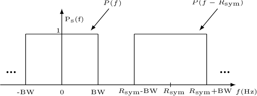
The Fourier pair $δ(t) ⇔ 1$ indicates that the property $p_{s} (t) = δ(t)$ is equivalent to having $P_{s} (f) = 1$ or some other constant.¹⁰ Because $P(f)$ determines $P_{s} (f)$ , the question now is what property of the shaping pulse $P(f)$ leads to $P_{s} (f) = 1$ . In other words, the Nyquist criterion can be derived by interpreting the desired property $p_{s} (t) = δ(t)$ in the frequency domain.

The spectrum of $P_{s} (f) = F{p_{s} (t)}$ is obtained by convolving $P(f)$ with $F{∑_{n=−∞}^{∞} δ(t − n T_{sym})}$ , the Fourier transform of the periodic impulse train. From Eq. (A.58), one has

P_{s} (f) = \frac{1}{T_{sym}} ∑_{k=−∞}^{∞} P (f − k \frac{1}{T_{sym}}) .

(4.24)

To have $P_{s} (f)$ with a constant value over all frequencies, Eq. (4.24) suggests that the replicas of $P(f)$ should gracefully compose this constant level when summed up and, there should be no gaps (frequencies for which $P_{s} (f) = 0$ ) among the replicas.

Assuming $P(f)$ is the spectrum of a bandlimited baseband pulse with bandwidth $BW$ and support from $− BW$ to $BW$ , it suffices to observe the interaction between $P(f)$ and its first replica at the right (positive frequencies), located at $P(f − R_{sym})$ . The support of $P(f − R_{sym})$ is from $R_{sym} − BW$ to $R_{sym} + BW$ and, as indicated in Figure 4.20, to avoid a gap of $P_{s} (f) = 0$ between the two replicas, it is mandatory to have $BW ≥ R_{sym} − BW$ . Therefore, for a baseband real signal, the Nyquist criterion for zero ISI is

R_{sym} ≤ 2 BW .

(4.25)

This criterion indicates that a channel with bandwidth $BW$ limits the symbol rate to $2 BW$ .

Figure 4.20: Explanation of the Nyquist criterion: the replicas of $P(f)$ for $k = 0$ and 1 in Eq. (4.24) cannot have a gap between them.

Example 4.9. Reasoning that leads to the Nyquist criterior for zero ISI. To illustrate Eq. (4.25), Figure 4.21 shows the replicas of $P(f)$ , spaced by $R_{sym}$ , that compose $P_{s} (f)$ . In this case, the bandwidth $BW = 200$ Hz of $P(f)$ is not large enough, and the gaps (where $P(f) = 0$ ) between the replicas indicate that it is not possible to obtain $P_{s} (f) = 1$ .

Figure 4.21: Spectrum of $P_{s} (f)$ corresponding to a $p(t)$ with a triangular spectrum $P(f)$ of $BW = 200$ Hz and $R_{sym} = 500$ bauds.

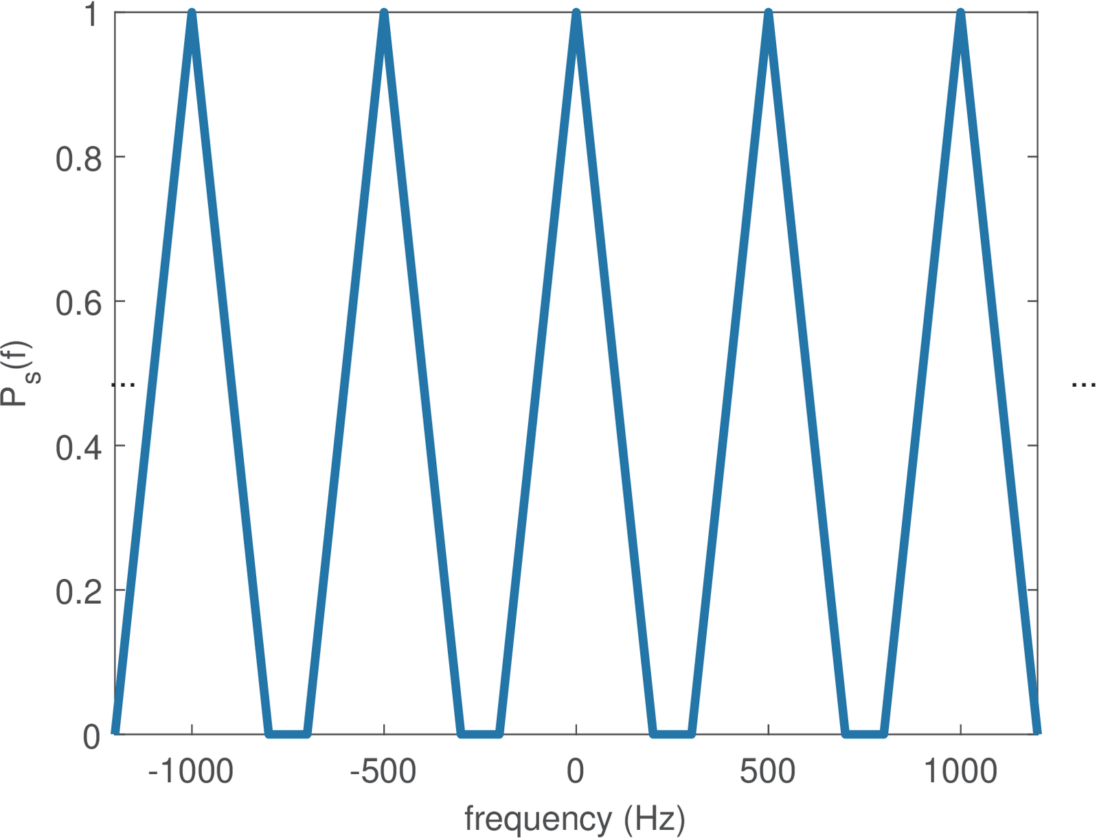
In fact, changing the triangular spectrum by a rectangular spectrum $P(f)$ with $BW = R_{sym} ∕2$ , one can achieve $P_{s} (f) = 1,∀f$ , which is the pulse with smallest $BW$ that achieves zero ISI. Several other options for $p(t)$ can achieve zero ISI. $□$

As further discussed in Table 4.3, for an analytic signal representing a bandlimited complex envelope (e. g., the one in Figure 3.6) with bandwidth $BW$ and $P(f)$ with support from $0$ to $BW$ , Eq. (4.25) becomes

R_{sym} ≤ BW .

(4.26)

Zero ISI with a discrete-time model

The discrete-time model of Block (2.16) is adopted now and the emphasis is on showing some code, while equations were prioritized when discussing the continuous-time model. Assuming $L$ is the oversampling in Block (2.16), the desired property for the shaping pulse $p[n]$ to achieve zero ISI is:

p[nL] = {\begin{matrix} 1, n = 0 \\ 0, n≠0 \end{matrix}

and the periodic impulse train is $x[n] = ∑_{k=−∞}^{∞} δ[n − kL]$ .

Some delay $N_{0}$ can be assumed, for example, to avoid non-causal pulses. In this case, the desired property is

p[nL+ N_{0}] = {\begin{matrix} 1, n = 0 \\ 0, n≠0 \end{matrix}

and the receiver should find the correct instant to start sampling at the symbol rate.

Because $x[n]$ has period $L$ , a natural tool to observe its spectrum is the discrete-time Fourier series. But it is convenient to use the DTFT for the spectra of both signals: $p[n]$ and $x[n]$ . The DTFT of $x[n]$ is another impulse train

X(e^{j Ω}) = \frac{2π}{L} ∑_{k=−∞}^{∞} δ (Ω + k \frac{2π}{L})

(recall that continuous-time impulses can be used to represent the spectrum of a periodic signal when one is interested in representing it as a Fourier transform instead of a Fourier series). The spectrum of $p_{s} [n] = p[n] × x[n]$ is

P_{s} (e^{j Ω}) = P(e^{j Ω})∗X(e^{j Ω}) = \frac{2π}{L} ∑_{k=0}^{L−1} P(e^{j(Ω +k \frac{2π}{L})}).

(4.27)

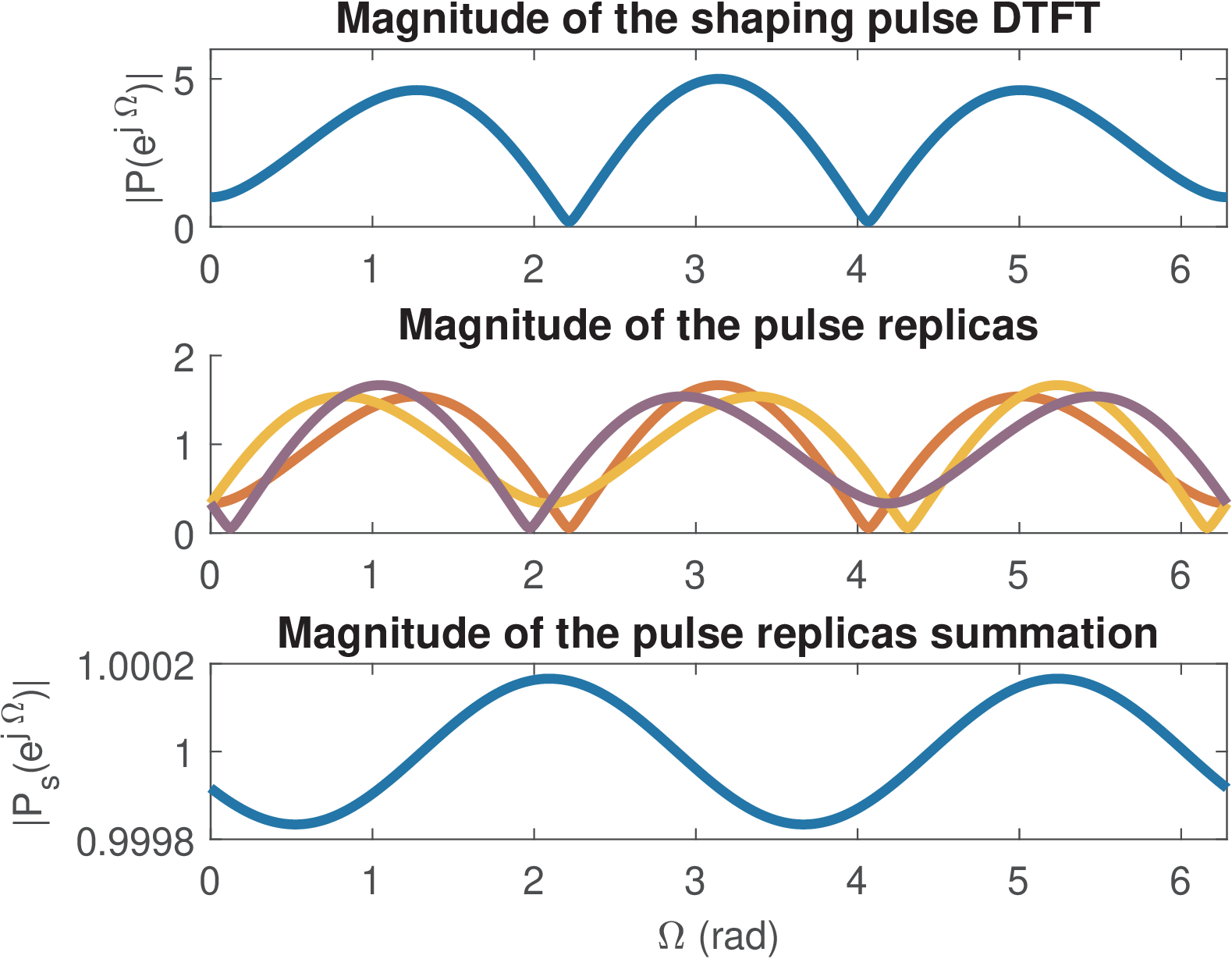
Example 4.10. Example of Nyquist pulse with support not longer than oversampling $L$ . The function ak_plotNyquistPulse.m can be used to observe that Eq. (4.27) leads to a constant value when the pulse obeys the criterion. Figure 4.22 shows the obtained spectra for a pulse p=[1 1 1 1] with $L = 4$ , using Listing 4.4.

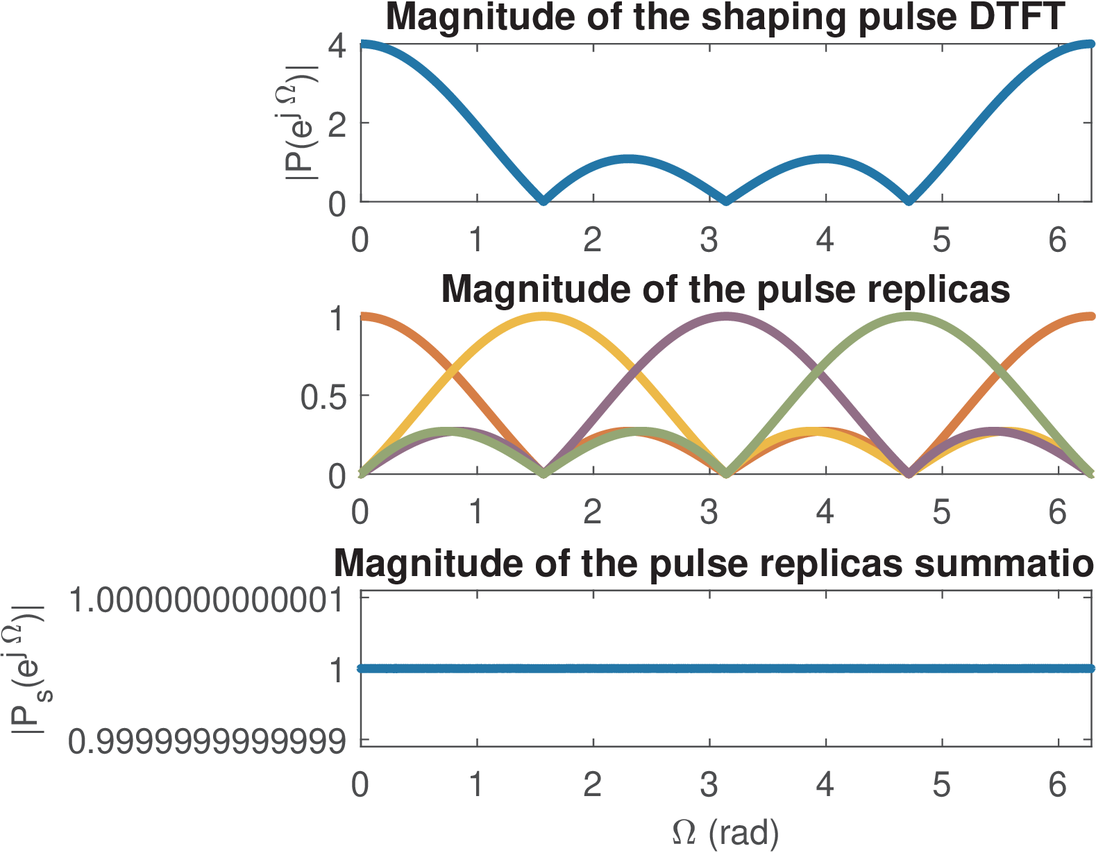
Figure 4.22: Spectra for the pulse p=[1 1 1 1]. From top to bottom: $P(e^{j Ω})$ , the $L = 4$ replicas of $P(e^{j Ω})$ that compose $P_{s} (e^{j Ω})$ and $P_{s} (e^{j Ω})$ itself. All the graphs are periodic and the shown interval is $Ω = [0,2π]$ rad.

Listing 4.4: MatlabOctaveCodeSnippets/snip_digi_comm_ak_plotNyquistPulse.m

1N0 = 1; %sample to start obtaining the symbols 
2p=[1 1 1 1]; %shaping pulse 
3L=4; %oversampling factor 
4ak_plotNyquistPulse(p,L) %graphs in frequency domain

Note the pulse has non-zero samples only for $n = 0,1,2,3$ and the oversampling is $L = 4$ . Hence, it should be expected no ISI in this case. The top and bottom plots in Figure 4.22 show $P(e^{j Ω})$ and $P_{s} (e^{j Ω})$ , respectively. The plot in the middle illustrates that, according to Eq. (4.27), for $L = 4$ there are four replicas of $P(e^{j Ω})$ that sum up to compose $P_{s} (e^{j Ω})$ .

Figure 4.23: Assuming the transmitted symbols are symbols=[3 -1 3 1], p=[1 1 1 1] and $L = 4$ , from top to bottom: $p[n]$ , the shifted and scaled versions of $p[n]$ corresponding to each symbol and the transmitted signal $s[n]$ .

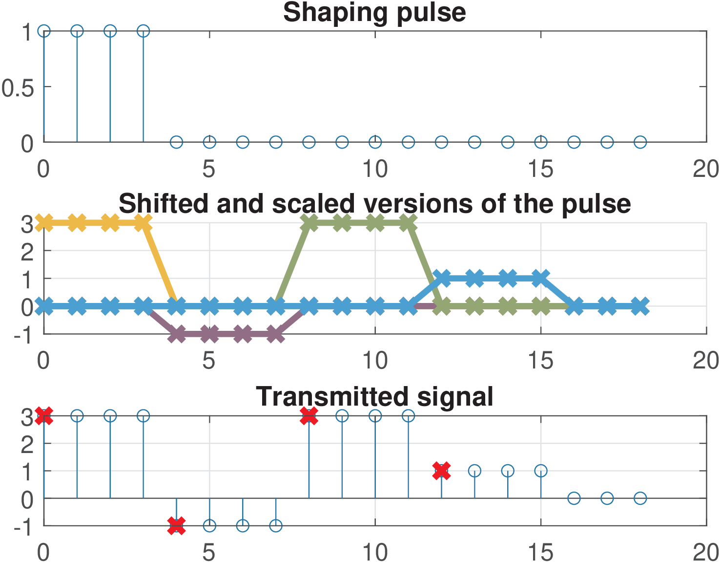
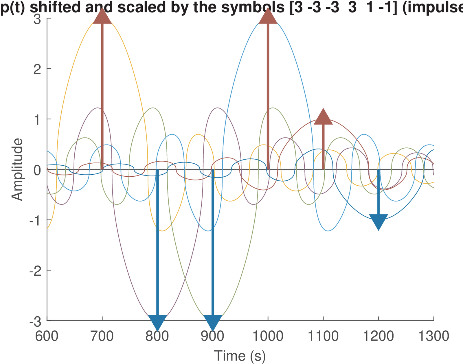
Besides Figure 4.22, it is instructive to analyze the pulse p=[1 1 1 1] (or $p[n]$ ) in time-domain. This is the goal of Figure 4.23, which shows $p[n]$ on the top graph. Assuming the transmitted symbols are symbols=[3 -1 3 1], the bottom plot shows the result of the convolution between the upsampled symbols and $p[n]$ , which corresponds to the transmitted signal. This graph shows the sampling instants, where the symbols can be recovered, as specified by N0 = 1. The middle graph shows the effect of shifting $p[n]$ and scaling it by the corresponding symbol. For example, the parcel corresponding to the first symbol is $3p[n]$ . Note that for $n = 0,4,8,12$ , there is only one parcel that has a non-zero value, as requested for zero ISI. $□$

Example 4.11. Example of Nyquist pulse with support longer than oversampling $L$ . As previously discussed, it is possible to use a pulse with duration longer than $L$ samples and still achieve zero ISI. This is useful in practice because a longer shaping pulse (think it as a FIR filter) can have sharper transitions from passband to stopband, which will determine the effective filter’s bandwidth. To exemplify this possibility, it is assumed a pulse p=[0 -1 2 1 1 -2 0], oversampling $L = 3$ and ak-here Figure 4.24 and Figure 4.25 were then obtained with Listing 4.5.

Figure 4.24: Equivalent to Figure 4.22 with the pulse p=[0 -1 2 1 1 -2 0].

Figure 4.25: Equivalent to Figure 4.23 with the pulse p=[0 -1 2 1 1 -2 0].

Listing 4.5: MatlabOctaveCodeSnippets/snip_digi_comm_ak_plotNyquistPulse2.m

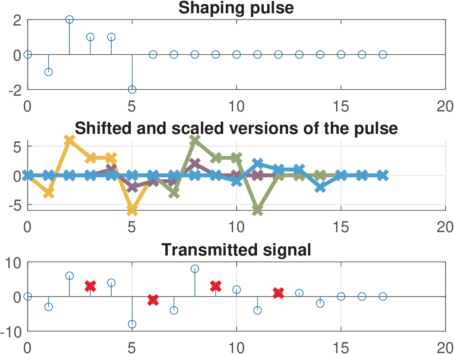
1N0 = 4; %sample to start obtaining the symbols 
2p=[0 -1 2 1 1 -2 0]; %shaping pulse 
3L=3; %oversampling factor 
4ak_plotNyquistPulse(p,L) %graphs in frequency domain

It is not that evident, but Figure 4.25 indicates that the ISI is zero. Its bottom graph informs that the four symbols $3,−1,3,1$ were perfectly recovered at samples $n = 3,6,9,12$ . The value N0=4 leads to the first symbol being obtained at $n = 3$ (N0-1). The bottom graph of Figure 4.24 shows that $P_{s} (e^{j Ω})$ is a constant over $Ω$ , with a numerical error of $± 0.0002$ .

Careful observation of the middle graph of Figure 4.24 indicates that, considering only the magnitude, the $L = 3$ replicas of $P(e^{j Ω})$ do not sum to a constant. Due to the delay imposed by N0, the phase must be taken in account, which was not necessary in Figure 4.22. $□$

As discussed in Application 4.3, there is considerable flexibility for designing zero ISI pulses. But, in practice, two requirements are imposed when interpreting the pulse as a filter: 1) a relatively small bandwidth and 2) a large attenuation at the stopband. The raised cosines are popular options and are discussed in the sequel.

4.4.6 Cursor, precursor ISI and postcursor ISI

The cursor was briefly mentioned in Section 2.12.3. Generally, given a signal waveform, a reference time instant is sometimes called cursor. The segments of the signal before and after this point are called precursor and postcursor, respectively. The next paragraphs, apply the concept of cursor in the specific scenario of a digital receiver, in which it is also called synchronization delay, timing synchronization delay, or delay due to timing synchronization.

Considering again the transmitted and received signals in Figure 2.5 and Figure 2.6, respectively, note that it is not trivial to find the instant to sample the signal at the receiver (or the cursor) given a distorted signal, as in Figure 2.6.

Before defining the cursor more accurately, it is useful to observe in Figure 4.26, two examples of channel pulse responses to a single symbol (“one-shot”) of a PAM signal $x(t)$ . In this case $p(t)$ in case (a) spans approximately $2.5 T_{sym}$ and potentially causes less ISI than case (b).

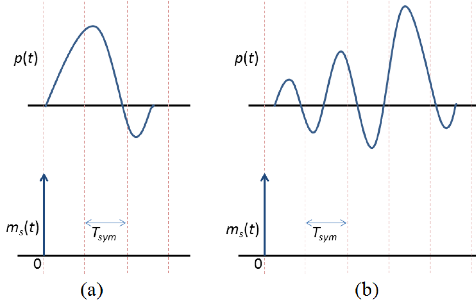
Figure 4.26: Two examples of channel pulse responses $p(t)$ : the second one, (b), potentially leads to stronger ISI due to its more dispersive channel than (a).

The timing references in Figure 4.26, with vertical lines separated by $T_{sym}$ have the transmitted signal as reference. In the context of ISI analysis, it is sometimes convenient to have the timing specified by the receiver synchronizer as indicated in Figure 4.27.

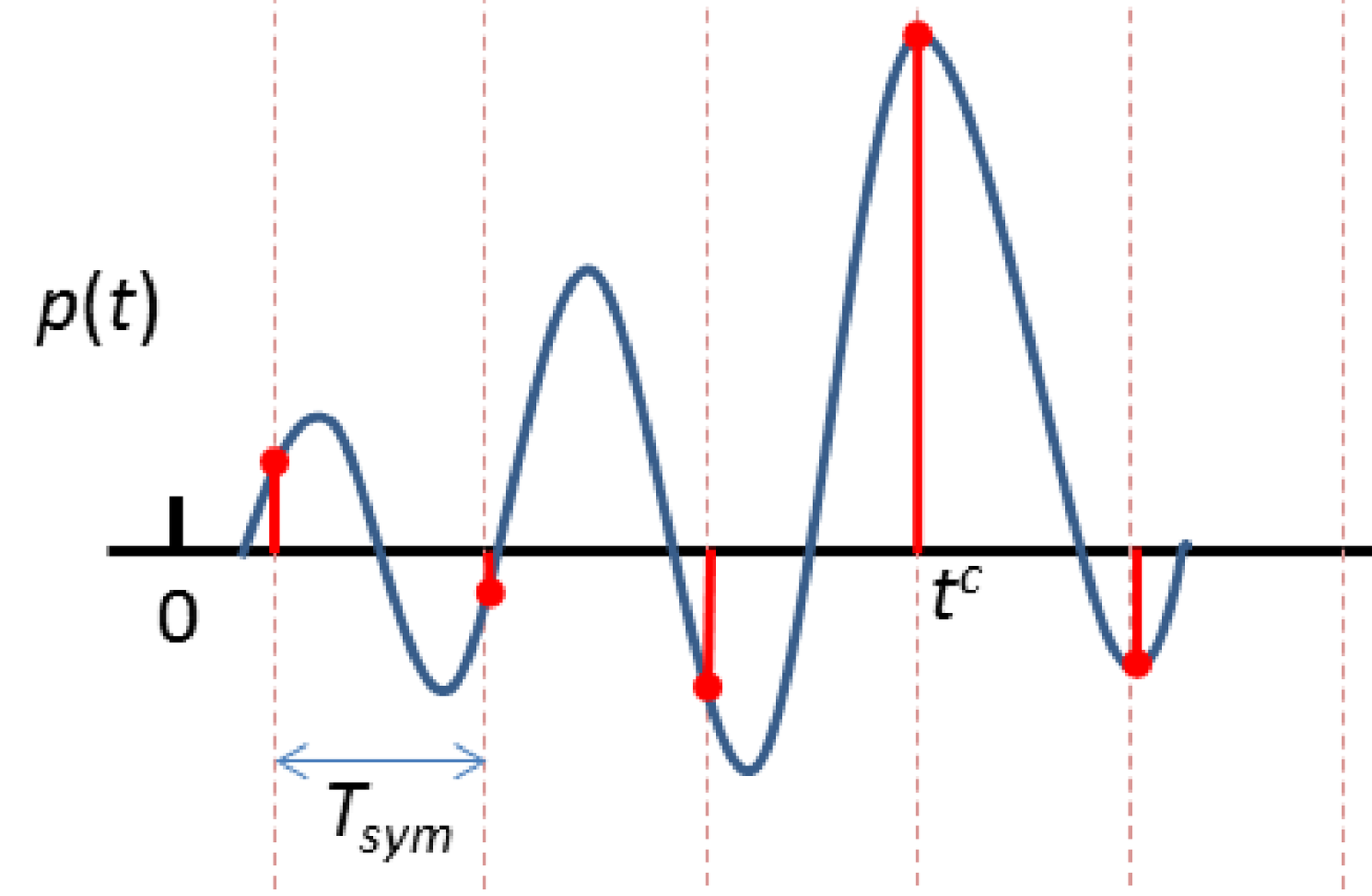
Figure 4.27: Pulse response of Figure 4.26(b) with the timing reference provided by the estimated cursor at $t^{c}$ .

Figure 4.27 indicates the cursor time $t^{c}$ (or simply cursor), which is typically estimated by the receiver’s synchronization algorithm. For a given reference symbol $m$ , the cursor is defined here as the time delay between the instant $m$ was generated at the transmitter and the time estimated by the receiver to obtain the amplitude value that will represent $m$ and be used for making the decision regarding the symbol. Considering distinct symbols $m[n]$ as the reference (time “0”), the estimated cursor values $t^{c} [n]$ may vary, and $t^{c} = 𝔼 [t^{c} [n]]$ is their average.

Assuming the signal that will be used at receiver to make the decisions is already at the symbol rate $R_{sym}$ , the samples of the pulse response $p(t)$ separated by $T_{sym}$ from $t^{c}$ may impact the decision of other symbols. In Figure 4.27, three samples before the cursor $t^{c}$ (precursor samples) may impact the three symbols that are transmitted before the reference symbol, while the sample at time $t^{c} + T_{sym}$ impacts the symbol transmitted just after the reference symbol. This is an important aspect of ISI that can be summarized as follows:

Precursor: interference provoked by future symbols, which can be modeled as anticausal with respect to the reference symbol, and it is created by the parcels of $p(t)$ before the cursors of the future symbols.
Postcursor: interference provoked by past symbols and created by the parcels of $p(t)$ after the cursors of the past symbols.

An example using $p(t)$ from Figure 4.26(a) is described in the next paragraphs.

Because the channel is LTI, it is relatively easy to observe its response to a sequence of symbols and interpret the final $p(t)$ as the summation of the contribution of each symbol. Figure 4.28 illustrates a case with four PAM symbols composing $m_{s} (t)$ and the corresponding responses that should be added to compose $p(t)$ .

Figure 4.28: Illustration of ISI at cursor $t^{c}$ corresponding to the symbol transmitted at $t = 2 T_{sym}$ (third symbol, in red). The adopted pulse response is from Figure 4.26(a).

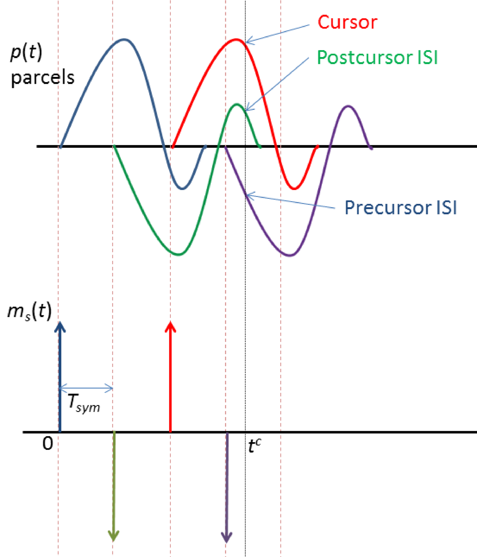
Observing Figure 4.28, suppose that the automatic synchronization procedure chooses $t^{c} [2]$ (or $t^{c}$ for simplicity) as the indicated cursor to obtain the sample that represents the symbol transmitted at time $2 T_{sym}$ . In this example, the signal at $t^{c}$ is the summation of three parcels: the parcel of interest, the precursor ISI (which in this case is provoked solely by the next symbol sent at $t = 3 T_{s}$ ) and the postcursor ISI (provoked by the previous symbol, transmitted at $t = T_{sym}$ ). In this case, only the two neighboring symbols are interfering with the reference symbol but, in general, due to the channel dispersion, it is possible that the symbol of interest suffers interference from many other symbols. As mentioned, the influence of “future” symbols can be conveniently modeled using noncausal signals and systems.

⁶ As discussed in Section 4.4.4, $p(t)$ is sometimes considered to be the shaping pulse $p_{t} (t)$ .

⁷ The nomenclature is based on [Cio10] (chapter about equalization).

⁸ Fourier theory explains that if $p(t)$ has finite support, its spectrum $P(f)$ cannot have and vice-versa. In other words, if $p(t)$ has finite duration, $P(f)$ has infinite bandwidth and if $P(f)$ is band limited then $p(t)$ has infinite duration. But in practice, functions can have negligible values outside ranges and, for practical purposes, be considered to have finite support in both time and frequency domains.

⁹ In practice, scaling factors are always necessary and often provided by closed-loop control systems (such as an automatic gain control system) within the transceiver circuitry.

¹⁰ Again: scaling factors are useful to get the right analytical results but in practice they depend on the electronics.