3.8  Orthogonal Modulations and FSK

Among the several modulations that use a linear combination of basis functions ${\phi }_i(t)$, according to Eq. (2.29), the orthogonal modulations are a special case in which the resulting signals $s_n(t)$ themselves are orthogonal when representing distinct signals. Consequently, the orthogonality can also be observed in the constellation diagram. Some of the most popular orthogonal modulations are FSK, PPM (pulse-position modulation) and PWM (pulse-width modulation).³

The frequency-shift keying (FSK) modulation was briefly discussed in Section 2.8. In FSK, each basis function corresponds to a sinusoid with a distinct frequency and the symbol is identified solely by the frequency of its basis function. A FSK system with $N$ dimensions has $M=N$ distinct symbols and the $i$-th symbol (coefficient), $i=0,\dots ,M-1$, can be represented by the vector ${\mathbf{\text{X}}}_i=[0,\dots ,0,1,0,\dots ,0]$, where the non-zero element is at the $i$-th position. The example of a discrete-time binary FSK system can clarify.

Assume a binary FSK system where $L=32$ samples. Figure 2.13 depicts an example. The bits 0 and 1 (called space and mark, respectively) are represented here by orthonormal sinusoids $\sqrt{\frac{2}{L}}\text{cos}<!--FUNCTION\; APPLICATION-->(2\pi ∕N_{i}n)$, where $N_0=8$ and $N_1=4$, respectively. Using the notation discussed in Section 2.12.4, the symbol representing the bit 0 is ${\mathbf{\text{X}}}_0={[1,0]}^T$ and ${\mathbf{\text{X}}}_1={[0,1]}^T$. The following Matlab/Octave commands illustrate that the basis functions are orthogonal and show an example of modulation and demodulation when transmitting a bit 1.

1L=32;       %number of samples per symbol 
2N_0=8;     %period of sinusoid corresponding to bit 0 
3N_1=4;     %period of sinusoid corresponding to bit 1 
4n=(0:L-1)'; %time index 
5A=[cos(2*pi/N_0*n) cos(2*pi/N_1*n)]*sqrt(2/L); %inverse matrix 
6innerProduct=sum(A(:,1).*A(:,2)) %check if the columns are orthogonal 
7Ah=A'; %the pseudoinverse is the Hermitian 
8X=[0; 1];  %example of symbol for transmitting bit 1 
9x=A*X; %compose the signal in time domain 
10X=Ah*x  %demodulation at the receiver: recover the coefficient

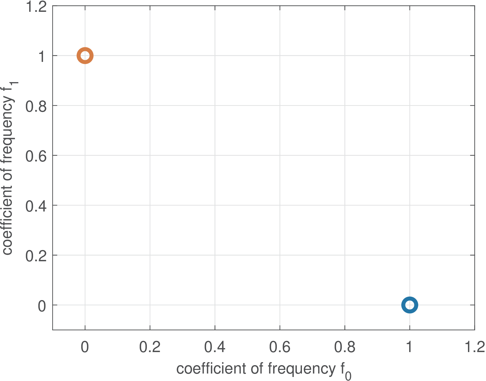
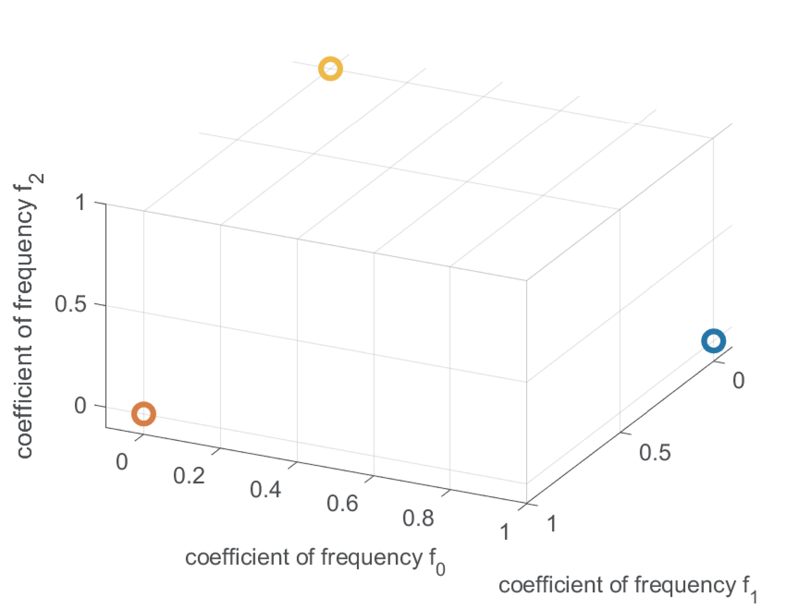
The constellation for a binary FSK is depicted in Figure 3.13. It has been emphasized that the orthogonality of basis functions is an important property. It can be noted that the FSK coefficient vectors themselves are orthogonal. Figure 3.14 presents a FSK constellation for $N=3$ dimensions. In this case the coefficients are ${[1,0,0]}^T$, ${[0,1,0]}^T$ and ${[0,0,1]}^T$, which form an orthonormal basis for ${ℝ}^3$. In contrast, the two basis functions of a QAM are orthogonal, but the coefficient vectors are not.

Application 3.1 gives more details of a binary FSK system.