Estimating Probability of Error for QAM

5.6 Estimating Probability of Error for QAM

The easiest QAM to analyze is the “squared” (SQ) $M$ -QAM, where the number $b = {log}_{2} M$ of bits is an even integer and the QAM constellation was obtained by the Cartesian product of two PAM constellations of $2^{b∕2} = \sqrt{M}$ symbols each. For example, two 2-PAMs with symbols $[−1,1]$ can be used to obtain a 4-QAM with symbols $[1,j,−1,−j]$ . In this case, the analysis is simplified by observing that PAM uses $D = 1$ dimension while QAM uses $D = 2$ dimensions, and the expressions “per dimension” are equivalent. For example, when using QAM, the filtered AWGN has a variance of $σ^{2}$ per dimension, such that the total noise power is $2 σ^{2}$ but the noise “per dimension” is the same as when using a PAM.

Table 5.1: Expressions for PAM and SQ QAM, where the M-QAM is obtained by the Cartesian product of two

\sqrt{M}

-PAM constellations.


	$M$ -PAM	SQ $M$ -QAM

$\bar{E_{c}}$	$\frac{d^{2}}{12} (M^{2} − 1)$	$\frac{d^{2}}{12} (M − 1)$

$\frac{d}{2σ}$	$\sqrt{\frac{3}{M^{2} −1} SNR}$	$\sqrt{\frac{3}{M−1} SNR}$

The SQ QAM constellation has energy given by

E_{c} = \frac{d^{2} (M − 1)}{6}

and the energy “per dimension” is $\bar{E_{c}} = E_{c} ∕N = E_{c} ∕2$ . This energy can be obtained from Eq. (2.10) by noting that one dimension has the energy of a $\sqrt{M}$ -PAM:

\bar{E_{c}} = \frac{d^{2} ({\sqrt{M}}^{2} − 1)}{12} = \frac{d^{2} (M − 1)}{12} .

A similar reasoning can be applied to other expressions: when a $M^{2}$ appears in a PAM expression, it changes to $M$ in the equivalent per dimension SQ QAM expression and a $M$ in PAM changes to $\sqrt{M}$ in the SQ QAM. Table 5.1 gives two examples.

Hereafter, an over line will be used to denote “per dimension” quantities. For example, the SER “per dimension” is

\bar{P_{e}} = P_{e} ∕N

and the number of bits per symbol per dimension is

\bar{b} = b∕N.

The exact probability of error expressions for SQ $M$ -QAM is

\begin{array}{l} P_{e} & = 4 (1 − \frac{1}{\sqrt{M}}) Q (\frac{d}{2σ}) − 4 {(1 − \frac{1}{\sqrt{M}})}^{2} {(Q (\frac{d}{2σ}))}^{2} \\ = 4 (1 − \frac{1}{\sqrt{M}}) Q (\sqrt{\frac{3 SNR}{M − 1}}) − 4 {(1 − \frac{1}{\sqrt{M}})}^{2} Q {(\sqrt{\frac{3 SNR}{M − 1}})}^{2} \end{array}

Discarding the term $Q {(⋅)}^{2}$ , which is typically very small, an approximated probability of error expression for SQ $M$ -QAM is

{\bar{P}}_{e} ≤ 2 (1 − \frac{1}{2^{\bar{b}}}) Q (\frac{d}{2σ}) = 2 (1 − \frac{1}{2^{\bar{b}}}) Q (\sqrt{\frac{3}{M − 1} SNR})

(5.12)

Note that the expression below is exact for PAM and a good approximation for QAM:

{\bar{P}}_{e}^{QAM} ≈ P_{e}^{PAM} = 2 (1 − \frac{1}{2^{\bar{b}}}) Q (\frac{d}{2σ}) .

(5.13)

Figure 5.8: QAM cross constellations for $b = 3,5,7$ and 9, from a) to d), respectively.

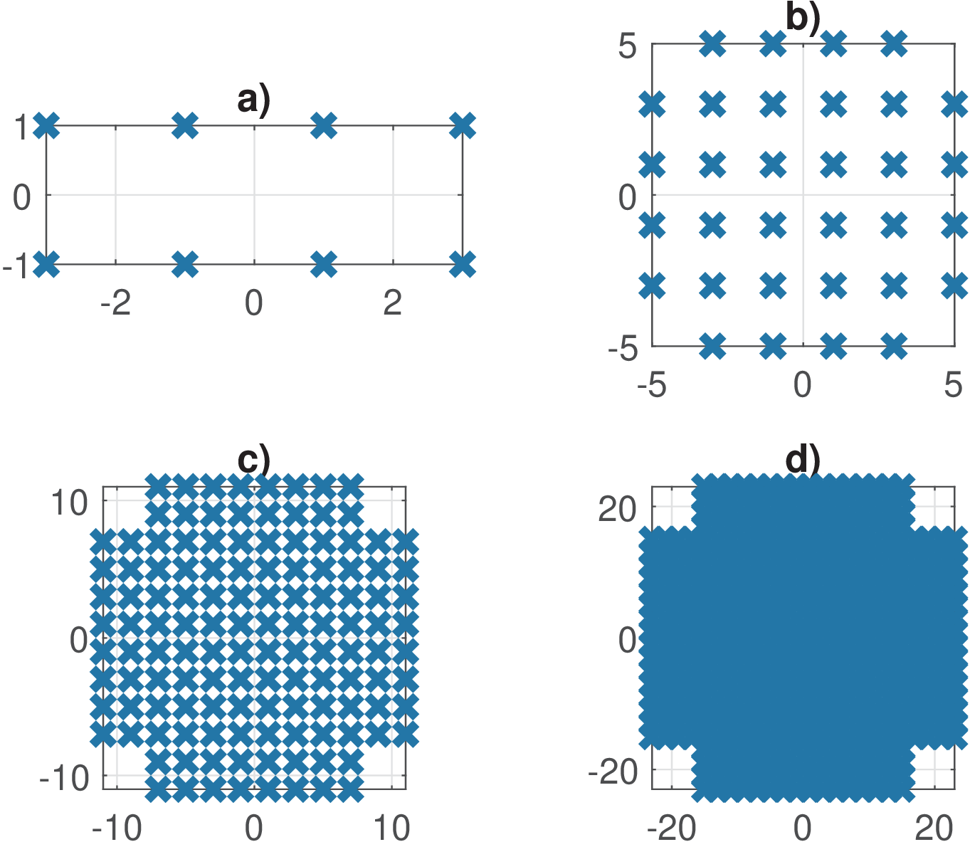
The previous analysis assumed SQ QAM, where $b$ is even and the constellation has the same number of symbols at both dimensions. When $b$ is odd, the constellation is typically organized as a “cross” and called CR QAM. Figure 5.8 illustrates four examples of CR QAM constellations.

The expressions for CR QAM (note that $D = 2$ ) are:

E_{c} = 2 \bar{E_{c}} = \frac{d^{2}}{6} (\frac{31}{32} M − 1)

\bar{b} = \frac{1}{2} {log}_{2} (\frac{32}{31} (12 \frac{\bar{E_{c}}}{d^{2}} + 1))

\bar{P_{e}} ≤ 2 (1 − \frac{1}{2^{\bar{b} +0.5}}) Q (\frac{d}{2σ}) = 2 (1 − \frac{1}{2^{\bar{b} +0.5}}) Q (\sqrt{\frac{3}{\frac{31}{32} (M − 1)} SNR}) .

5.6.1 Estimating probability of error for PSK

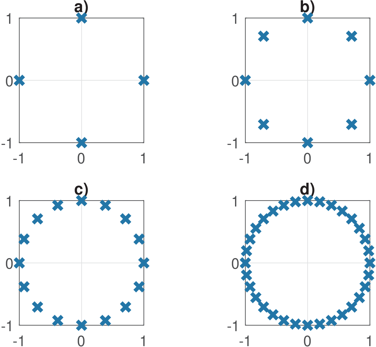
Figure 5.9: Examples of PSK constellations for $b = 2,3,4$ and 5 bits per symbol in a) to d), respectively.

The PSK modulation uses $D = 2$ dimensions but the information is conveyed only by the symbol phase because the symbol amplitude is constant. This is obtained by placing the constellation points with uniform angular spacing around a circle. PSK is often used when the channel imposes a nonlinear amplitude distortion. Figure 5.9 provides four example of $M$ -PSK constellations.

The binary PSK is called BPSK. The quaternary PSK uses $M = 4$ symbols and is called QPSK. It corresponds to a QAM and its $P_{e}$ can be obtained from the corresponding QAM expression. For a PSK other than BPSK and QPSK (i. e., for $M > 4$ ), there is no simple expression for the $P_{e}$ [ url5psk]. A relatively tight bound for PSK is

P_{e} < 2Q (\frac{\sqrt{E_{c}} sin (π∕M)}{σ}) .

Two important facts is that translating and rotating a constellation does not change $P_{e}$ . For example, the QAM constellations $[1,j,−1,−j]$ leads to the same $P_{e}$ as $\frac{\sqrt{2}}{2} [1 + j,−1 + j,−1 − j,1 − j]$ .

5.6.2 Statistical validity of error probability estimations

One needs to be careful when estimating the BER using a simulation that transmits bits and counts the errors at the receiver. This is called Monte Carlo simulation and requires a large number of bits when the BER is small. For example, when $P_{e} = 0.01$ , an error is expected to occur at each 100 transmitted bits, but only at each 10,000 transmitted bits if $P_{e} = 0.0001$ .

Figure 5.10: Comparison of simulated and theoretical BER for binary PAM (the result for BPSK is equivalent).

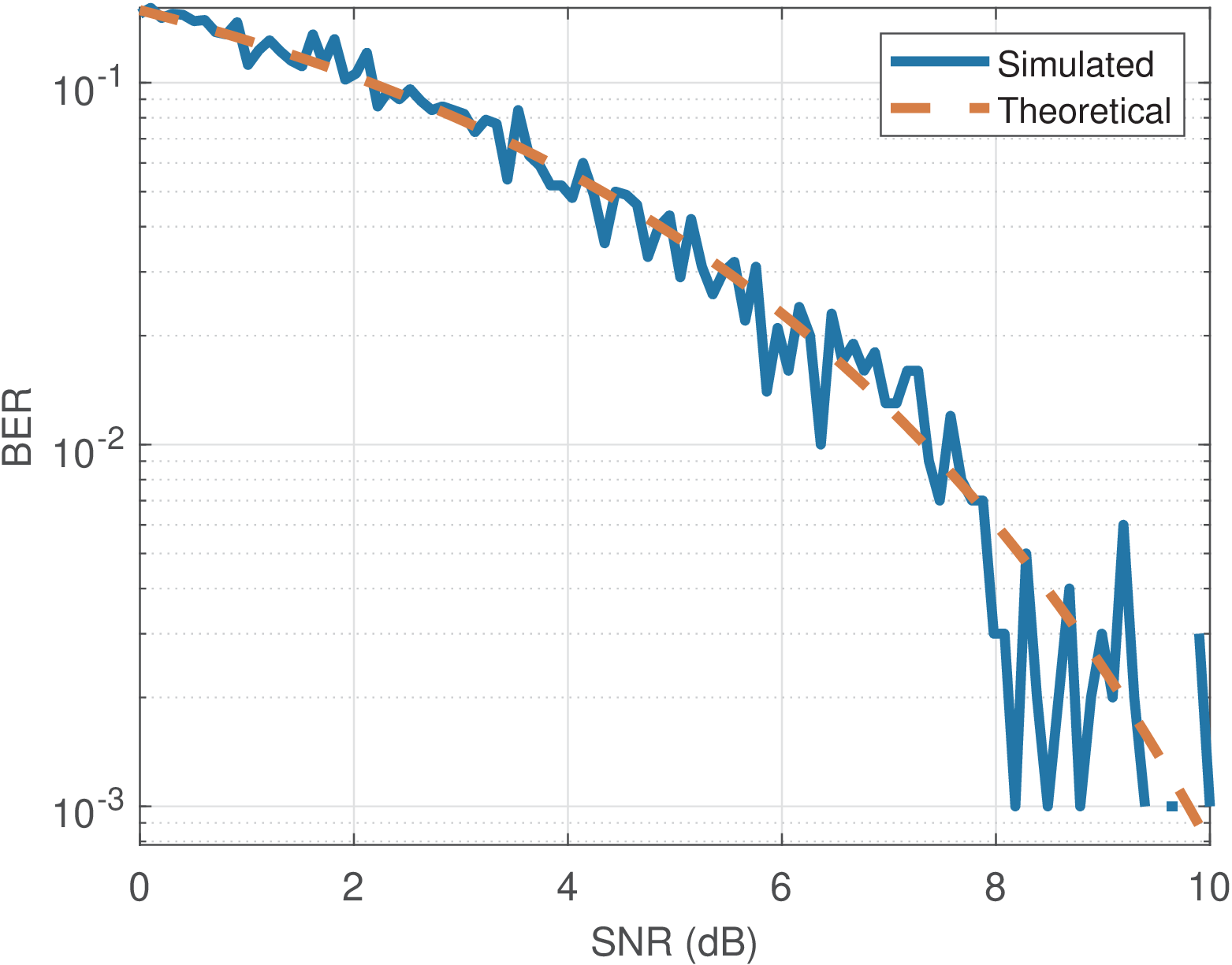
If there are no errors in a simulation using few bits, it does not necessarily mean that the actual BER is zero, but it may be the case that there were not enough bits in the transmitted signal. As a rule of thumb, 100 (or more) errors should occur in a simulation in order to have a robust estimate of the BER. In other words, if the expected BER is $P_{e}$ , a reasonable number of bits to be transmitted over the channel in a simulation to get a robust BER estimate is $100∕ P_{e}$ . At a high SNR, this can require transmitting millions, or even billions of bits. For example, when dealing with $P_{e} = 1 0^{−7}$ , the transmission of $100∕ P_{e} = 1 0^{9}$ bits should be planned. The code Listing 5.3 was used to generate Figure 5.10, which illustrates the issue.

Listing 5.3: MatlabOctaveBookExamples/ex_pam_ber.m

1%Perform a symbol-based simulation for binary PAM / PSK 
2d=20; %Distance between symbols 
3A=d/2; %Amplitude A=d/2 Volts 
4Nbits = 1000; %Number of transmitted bits 
5bits = rand(1,Nbits)>0.5; %bits (0 or 1) 
6symbols = A*2*(bits-0.5); %symbols (-A or A) 
7snr_dB = linspace(0,10,100); %SNR in dB 
8snr = 10 .^ (0.1*snr_dB); %linear SNR 
9noisePower = A^2 ./ snr; %noise power (sigma^2) 
10V=length(noisePower); %number of points in grid 
11ber = zeros(1,V); %pre-allocate space 
12for i=1:V 
13    %generate noise 
14    noise = sqrt(noisePower(i)) * randn(size(symbols)); 
15    %AWGN 
16    receivedSymbols = symbols + noise; 
17    %recover bits using ML threshold equal to 0 
18    decodedBits = receivedSymbols > 0; 
19    ber(i) = sum(decodedBits ~= bits)/Nbits; %estimate BER 
20end 
21%compare with theoretical expression: 
22if 1 %first option 
23    theoreticalBER = ak_qfunc(d ./ (2*sqrt(noisePower)) ); 
24else %second option 
25    theoreticalBER = ak_qfunc(sqrt(snr)); 
26end 
27clf, semilogy(snr_dB,ber,snr_dB,theoreticalBER,'--'); 
28xlabel('SNR (dB)'); ylabel('BER'); grid; 
29legend('Simulated','Theoretical');

Listing 5.3 used only Nbits = 1000 bits and the accuracy of the estimate became low when the SNR increased. This is expected because for $SNR = 10$ dB, the theoretical BER is smaller than $0.001$ and having no errors leads to the misleading estimate of $P_{e} = 0$ . In this case, reducing the maximum SNR or increasing the number of bits is mandatory for a robust estimate of $P_{e}$ .