Detection Theory and Probability of Error for AWGN Channels

5.2 Detection Theory and Probability of Error for AWGN Channels

One application of detection theory is choosing hypotheses given a set of measurements. In our case, the problem is to choose a symbol $m ∈ M$ given the received signal. Instead of dealing with waveforms, Listing 4.3 indicated that for AWGN and matched filtering it is appropriate to use a symbol-based simulation or, equivalently, adopt a vector channel model.

There are three basic aspects that define the estimation of symbol error probabilities:

f 1.: The noise distribution (power, dynamic range, etc.) at the receiver.
f 2.: The characteristics of the signal of interest at the receiver, given primarily by the transmitted constellation (position of symbols, constellation energy, probability of each symbol) and the energy of the shaping pulse.
f 3.: The decision regions used by the receiver, which typically depend on the adopted criterion, such as maximum likelihood (ML) or maximum a posteriori (MAP).

Because the following discussion assumes AWGN, it is sensible to also assume that a matched filter is used and adopt the notation of Section 4.3.4. But to simplify the expressions, it is considered unitary-energy pulses with $E_{p} = 1$ and scalar or complex symbols (not vectors with arbitrary $N > 2$ elements). This way the notation can rely on a symbol $m$ being transmitted and the receiver observing $r = m + z$ . This allows to abstract the whole process of creating a waveform via pulse shaping to transmit $m$ and recovering it at the receiver. The reader must be aware though that $r$ is obtained with a MF such that the receiver does not make the decision based on a single sample of the received signal.

Figure 5.3: Voronoi regions for a constellation with $M = 6$ symbols. The plot at the right highlights the decision region corresponding to symbol $[1,1]$ .

The receiver is assumed to choose a method for making decisions. This method could be eventually arbitrarily choosing thresholds to make decisions with if/else. But in practice, the receiver follows a sound mathematical method, such as making decisions to minimize the probability of symbol error $P_{e}$ .

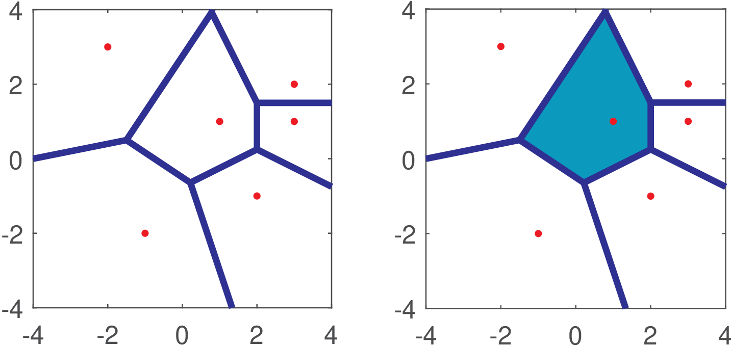
Given a decision method, the space where the transmitted $m$ (and received $r$ ) symbols rely is partitioned and each transmitted symbol $m_{i}$ becomes associated to a decision region $R_{i}$ . From the receiver’s perspective, all points belonging to $R_{i}$ will be interpreted as $m_{i}$ . For the sake of example, let $m_{i} ∈ M$ be a two-dimensional vector from the set $M = {[1,1],[3,2],[−1,−2],[−2,3],[2,−1],[3,1]}$ as in Figure 5.3. To provide better visualization, the symbols were on purpose arbitrarily positioned instead of using constellations adopted in practice. Assume the receiver makes decisions according to the minimum Euclidean distance criterion, which is equivalent to partitioning the space into decision regions called Voronoi regions as depicted Figure 5.3. For example, all received symbols $r$ that fall in the region associated to $[1,1]$ will be interpreted as $[1,1]$ .

The error probability $P_{e}$ depends on the decision regions and also on how the noise influences each symbol. The conditional probability of the output symbol $r$ given the input symbol $m$ , $p(r|m)$ completely describes the discrete-time AWGN (in fact, any vector channel). For AWGN, all conditional distributions $p(r|m)$ are Gaussians.

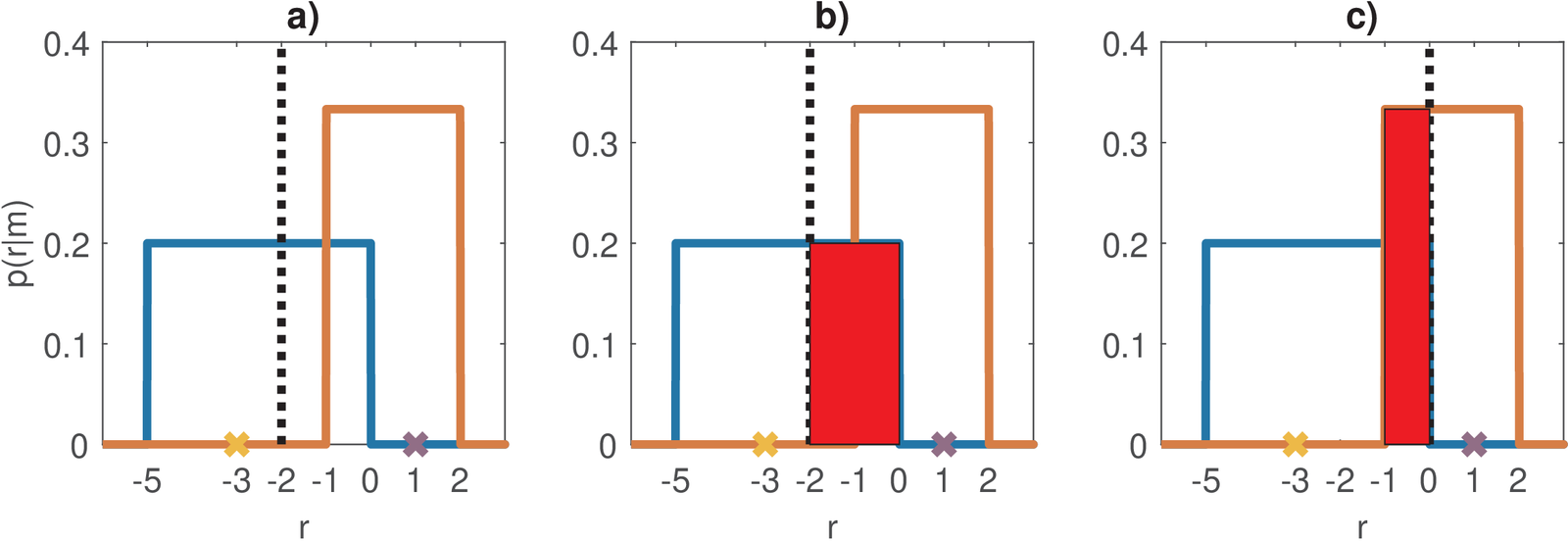
Figure 5.4: Conditional probabilities $p(r|m = −3) = U(−5,0)$ and $p(r|m = 1) = U(−1,2)$ for a binary transmission with symbols $m ∈{−3,1}$ . The decision threshold (indicated by a dotted line) is $γ = −2$ for a) and b), and $γ = 0$ for c). The areas in b) and c) indicate conditional error probabilities $p(e|m)$ .

As an example, assume a binary transmission with symbols $m ∈{−3,1}$ with prior probabilities 0.9 and 0.1, respectively. The noise is such that $p(r|m = −3) = U(−5,0)$ and $p(r|m = 1) = U(−1,2)$ are uniform distributions. The conventional AWGN is not used because it is simpler to calculate the probabilities with uniform rather than Gaussians PDFs. The receiver adopts a threshold equal to $γ = −2$ to create two decision regions. Figure 5.4 illustrates the example. The SER $P_{e}$ is given by

P_{e} = p(m = −3)p(e|m = −3) + p(m = −1)p(e|m = −1),

where $p(e|m)$ is the probability of error given that $m$ was transmitted. In this case, the noise that affects a transmitted $m = 1$ is never strong enough to cause an error, and $p(e|m = 1) = 0$ . When transmitting $m = −3$ , there is a chance that the received symbol falls in the range $[−2,0]$ , which is within the decision region of symbol $m = 1$ and these cases are wrongly interpreted. Hence, the $p(e|m = −3) = ∫_{−2}^{0} p(r|m = −3)dr = 2 × 0.2 = 0.4$ is given by the indicated area in Figure 5.4 b) and

P_{e} = 0.9 × 0.4 + 0.1 × 0 = 0.36.

The previous $P_{e}$ calculation assumed the receiver already had established the decision regions based on the threshold $γ = −2$ . A pertinent question is what is the optimal threshold to minimize $P_{e}$ ? Listing 5.2 can help finding the optimal $γ$ in this very specific case.

Listing 5.2: Brute-force method for finding optimal decision regions.

1N=1000; thresholds = linspace(-2,2,N); Pe = zeros(1,N); 
2for i=1:N %loop over the defined grid of thresholds 
3    Pe1=0.2*(-thresholds(i)); Pe2=1/3*(thresholds(i)+1); 
4    if Pe1<0 Pe1=0; end %a probability cannot be negative 
5    if Pe2<0 Pe2=0; end %a probability cannot be negative 
6    Pe(i) = 0.9*Pe1+0.1*Pe2;%prob. error for thresholds(i) 
7end 
8plot(thresholds, Pe); %visualize prob. for each threshold

Because the prior of $m = −3$ is much higher, the optimal threshold is 0 for this example, such that all transmitted symbols $m = −3$ are properly interpreted and $p(e|m = −3) = 0$ . The new situation with $γ = 0$ is indicated in Figure 5.4 c), with the highlighted area corresponding to $p(e|m = 1) = 1∕3$ . In this case,

P_{e} = 0.9 × 0 + 0.1 × 1∕3 = 1∕30.

In decision theory, the minimum achievable error (when using the optimal decisions) is called the Bayes error. In the digital communication scenario, the Bayes error is zero only when the conditional probabilities $p(r|m)$ do not overlap, which does not occur if they are Gaussians given their infinite support.

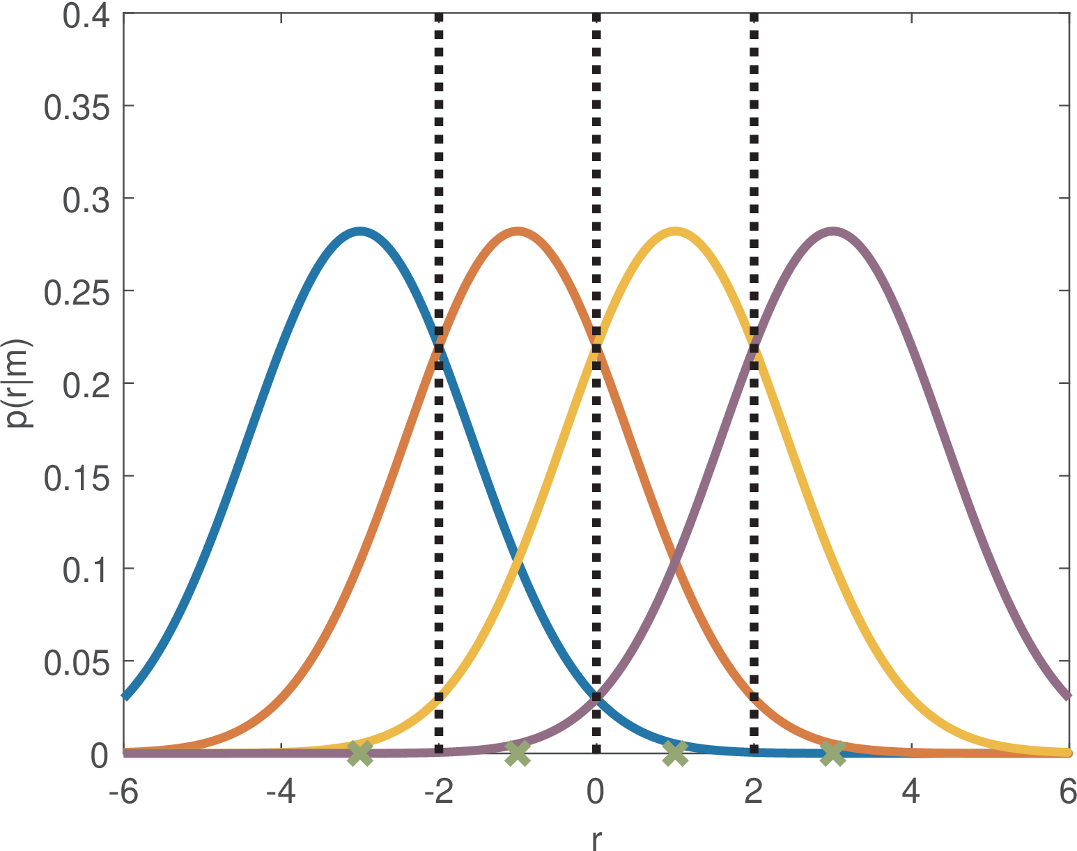
Figure 5.5: Conditional probabilities $p(r|m)$ for a 4-PAM with symbols $m ∈{−3,−1,1,3}$ assuming a Gaussian noise with variance $σ^{2} = 2$ .

For the AWGN case, and because in most cases the symbols are equiprobable, calculating $P_{e}$ via Eq. (5.1) can benefit from the symmetry of the problem. Figure 5.5 depicts $p(r|m)$ for a 4-PAM with symbols ${−3,−1,1,3}$ assuming a Gaussian noise with variance $σ^{2} = 2$ . In the discussion associated to Figure 5.2, $P_{e} = \frac{3Q(1∕σ)}{2}$ was already obtained for this 4-PAM case with AWGN. The next paragraphs seek a general result, valid for any PAM. In some situations, as this one, it is useful to use the probability of making correct decisions $P_{c}$ , given by $P_{c} = 1 − P_{e}$ . The reason is that sometimes the conditional $p(c|m)$ are easier to calculate and $P_{e}$ can be derived as

P_{e} = 1 − P_{c} = 1 − ∑_{m∈ M} P(m)P(c|m),

instead of using Eq. (5.1).

In the sequel, two criteria for defining the decision regions are presented.