What You Will Learn

5.1 What You Will Learn

This chapter discusses how to evaluate the symbol error probability for different modulation schemes when the channel is AWGN. For the AWGN there is no restriction on the signal bandwidth and the noise at the receiver is Gaussian, which simplifies calculations. Also, the optimal receiver for AWGN channels is discussed.

Some of the concepts are:

It is beneficial in terms of computational cost to use symbol-based instead of sample-based simulations.
The matched filter followed by an adequate sampling scheme is the optimum receiver for AWGN.
Matched filters and correlators are equivalent with respect to their output at the time instants of interest.
Decision criteria such as MLE and MAP impose decision regions and, consequently, the decision thresholds.

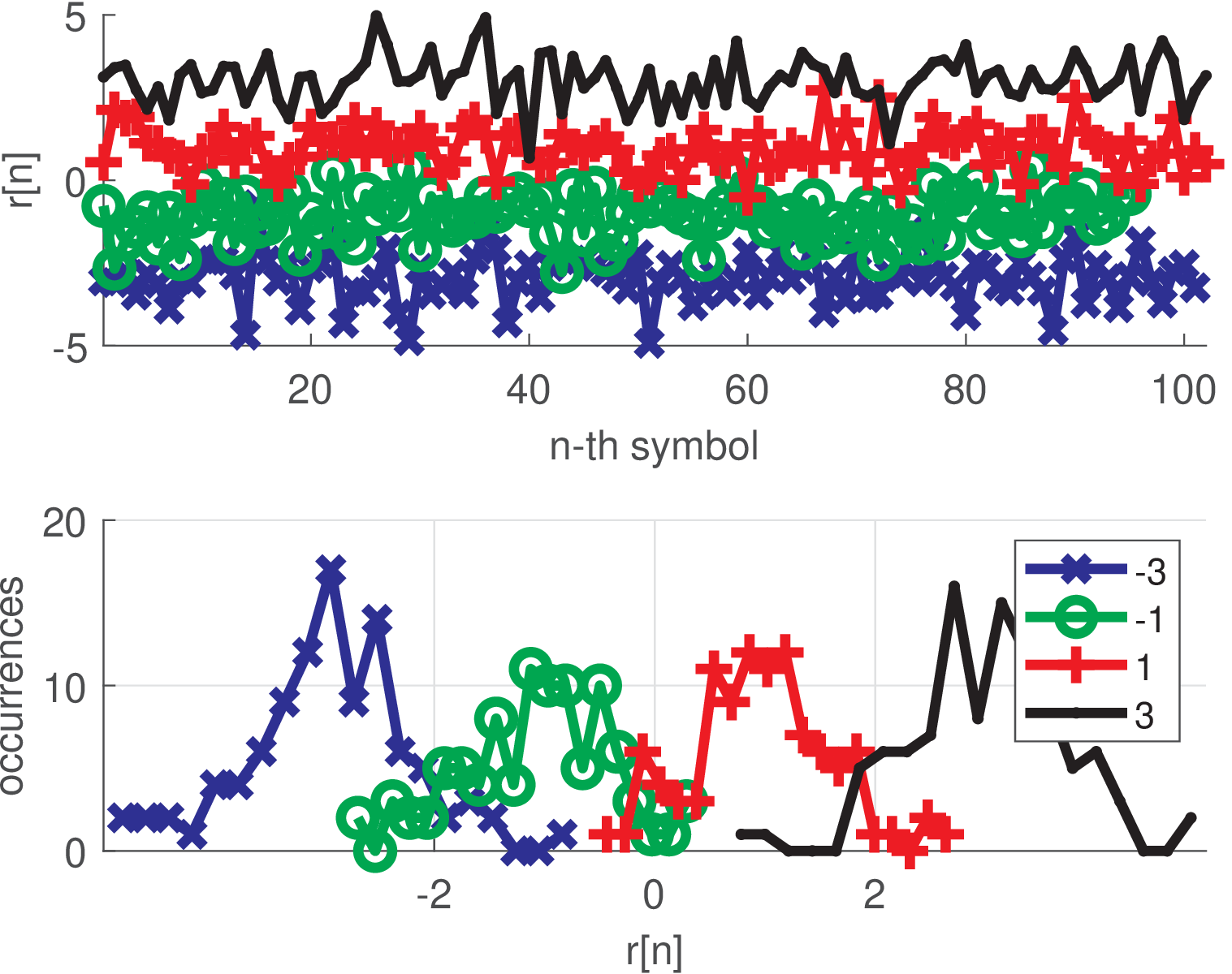
Figure 5.1: Received symbols of 4-PAM simulation at SNR of 10 dB, $P_{e} = 0.13$ and $P_{b} = 0.08$ . Each curve corresponds to a specific transmitted symbol. Top graph shows the symbols over time with each curve representing the corresponding symbols and bottom graph shows superimposed histograms.

Figure 5.1 shows a result obtained with the command

1ak_getErrorPDFsOfPAMWaveformSimulationInAWGN(100,8,4,0.5)

This function splits the received symbols according to the transmitted symbol, such that they can be interrelated. The simulation corresponding to Figure 5.1 used 4-PAM with equiprobable symbols constellation $− 3,−1,1,3$ , which gives an average energy of 5. The shaping pulse $p[n]$ has energy equal to the oversampling factor $L = 8$ , such that its power is unitary (in the continuous case, $p(t)$ would have energy $T_{sym}$ ). This implies that the signal has average power of 5. The noise power was 0.5, which corresponds to a SNR of approximately $10 {log}_{10} (5∕0.5) = 10$ dB. The number of transmitted bytes was 100, which corresponds to a total of $800∕2 = 400$ symbols, given that each symbol represents 2 bits. In spite of using rand.m for the distribution over the symbols, they are of course only approximately uniformly distributed. In the example, the symbol $− 1$ appears more times than the others. This histogram allows to calculate the error probability $P_{e}$ by observing the number of symbols that crossed the boundaries of the decision regions: $[−2,0,2]$ .

The simulated confusion matrix C for the example is indicated below:

     C = [91    10     0     0
          12    75     8     0
          0     7     89     6
          0     0      9    93]

where the element C $(m,n)$ corresponds to the number of occurrences of receiving the $n$ -th symbol after transmitting the $m$ -th symbol. The noise transformed 10 symbols “ $− 3$ ” into errors (interpreted as “ $− 1$ ”), while 12 symbols “ $− 1$ ” turned into “ $− 3$ ” and 8 into “1”. 13 and 9 are the number of errors for symbols “1” and “3”, respectively. Therefore, $P_{e} = (10 + 20 + 13 + 9)∕400 = 0.13$ is the estimated SER. Note the symbols “ $− 3$ ” and “3”, at the extrema of the constellation, lead to less errors than “ $− 1$ ” and “1”, because the latter have smaller regions due to the two neighbors. The adopted constellation uses a natural order such that the symbols $[−3,−1,1,3]$ are represented by the bits 00, 01, 10, 11. In this case, matrix C informs that the total number of bit errors is $10 + 12 + 2 × 8 + 2 × 7 + 6 + 9 = 67$ and the BER can be estimated as $P_{b} = 67∕800 = 0.08375$ . Gray coding could reduce the BER to $P_{b} = (10 + 12 + 8 + 7 + 6 + 9)∕800 = 0.065$ , achieving $P_{b} = P_{e} ∕b$ , which is the minimum BER for a given SER.

The next section aims at providing a gentle reasoning for the fact that after an AWGN channel, the PDF of the received symbol is a mixture of Gaussians positioned at the transmitted symbols.

5.1.1 Probability distribution of received signal at AWGN output

It is a convenient moment to practice modeling the statistics of the received symbols at the discrete-time AWGN output. Assume that, as in Section 2.13, the 4-PAM symbols are $− 3,−1,1,3$ and the AWGN noise is a random variable $N$ with zero mean and power equal to its variance $σ^{2} = 0.5$ , so its amplitude has a RMS value of $σ = \sqrt{0.5}$ .

For example, when symbol $m = −3$ is transmitted, the receiver observes a random amplitude $R = m + N$ that has the same PDF of $N$ but with the mean shifted by $m$ . Another way of looking at this result is recalling that the PDF of a sum of two independent random variables is the convolution of the input PDFs. The transmitted symbols compose a discrete random variable with a given PMF, which can be represented as a PDF via impulses located at the constellation points. The noise PDF is Gaussian and the convolution of the two PDFs generate a mixture of $M$ Gaussians, each one centered at the respective constellation symbol.

In this example and when symbol $m = −3$ is transmitted, an error occurs whenever $N > 1$ . Because there are no constellation symbols smaller than $− 3$ , i. e. $− 3$ is an “external” symbol with only one neighbor at its right (while $− 1$ and $1$ are “internal” symbols with two neighbors each). Hence, any noise value $N < 1$ does not cause errors when $− 3$ is the transmitted symbol. For example, even if the noise is $− 12$ , the received symbol would still be interpreted as $− 3$ . Hence, the probability $P(N > 1)$ of this error event is given by the Q function (see, Section ??), i. e., $P(N > 1) = Q(1∕ \sqrt{0.5}) ≈ 0.079$ .

Figure 5.2: PDFs of the noise $N$ with zero mean and variance $σ^{2} = 0.5$ and received symbol $R = m + N$ when symbol $m = −3$ is transmitted. The PDF of $R$ is a shifted version of the $N$ PDF.

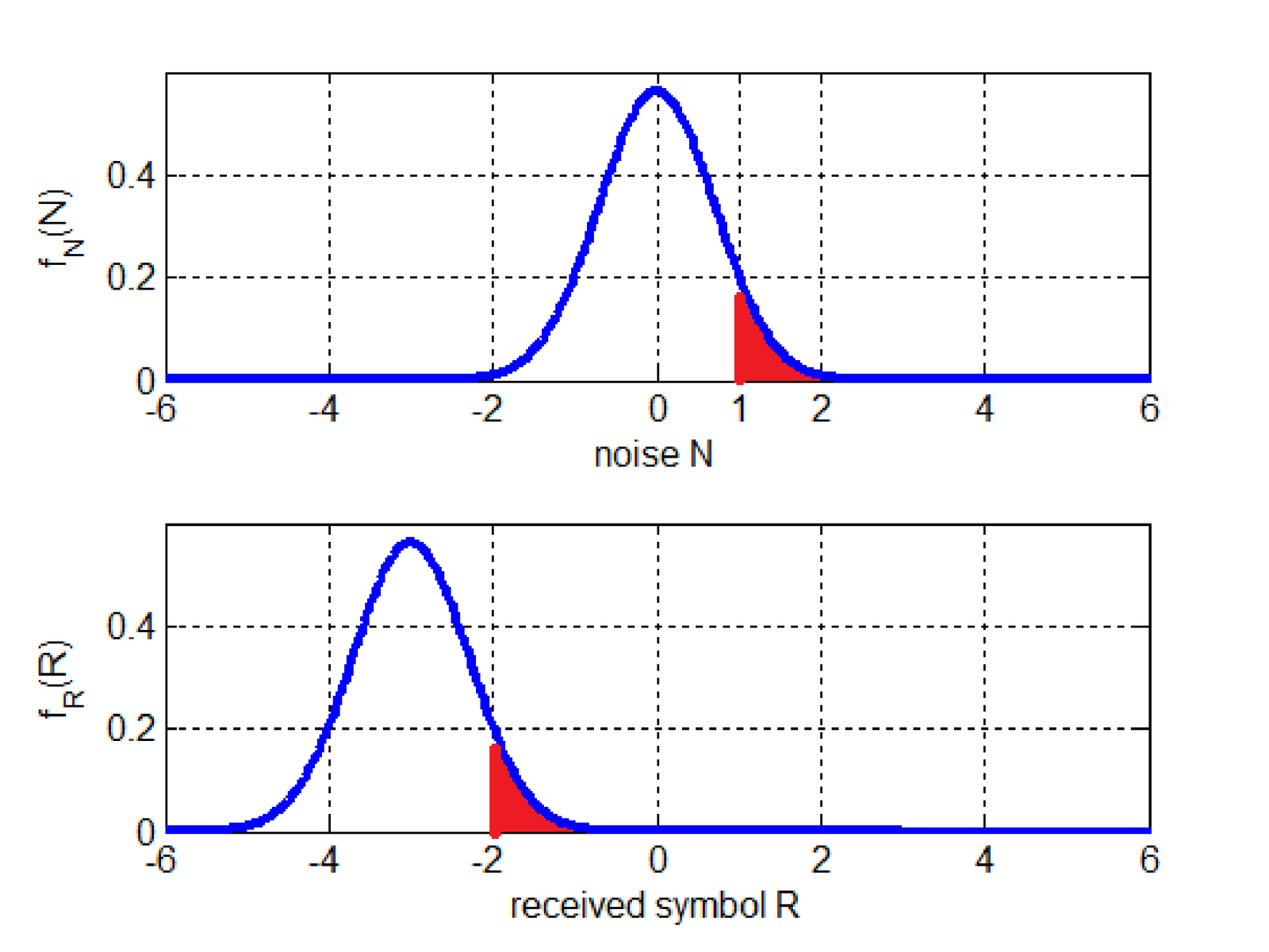
Recall that $Q(z)$ corresponds to the area under the tail of a standard normal¹ in the range $[z,∞[$ . When one wants to use $Q(z)$ for a non-normalized Gaussian with mean $μ$ and variance $σ^{2}$ to get the area on the interval $[x,∞[$ , it is necessary to normalize $x$ before invoking the function. In other words, when the received sample $R$ is distributed according to a Gaussian $N(R |μ,σ)$ ,

P(R > x) = Q (\frac{x − μ}{σ}) .

In the previous example, $μ = −3$ and the decision threshold is $x = −2$ , such that the error parcel has probability $P(R > x) = Q (\frac{−2−(−3)}{\sqrt{0.5}}) .$ Note that it is equivalent to calculating the tail of either $N$ or $R$ PDFs given that the decision threshold $x$ (for the range $[x,∞]$ ) is properly chosen. In the example, $P(R > −2) = P(N > 1)$ because $R = −3 + N$ . Figure 5.2 illustrates the concept using the red-colored area.

The calculated $P(N > 1) = Q(1∕ \sqrt{0.5})$ is conditioned on the transmission of symbol $m = −3$ and will be represented as the probability of error given that $m = −3$ was transmitted $P(e|m = −3)$ . The SER can be calculated as

P_{e} = ∑_{m∈ M} P(e,m)

and, because the events of sending distinct symbols are disjunct (cannot occur simultaneously):

P_{e} = ∑_{m∈ M} P(e,m) = ∑_{m∈ M} P(m)P(e|m),

(5.1)

where $P(m)$ is the symbol a priori probability.

The previous example assumed an external symbol $m = −3$ and concluded that $P(e|m = −3) = P(R > −2) = Q(1∕σ)$ . It is informative to calculate $P(e|m = 3)$ , corresponding to the other external symbol $m = 3$ .

Note that $P(e|m = 3) = P(R < 2)$ and a key point is to notice that the normalization $Q (\frac{x−μ}{σ})$ cannot be directly applied when one wants to get the area over the interval $] −∞,x]$ , i. e., the left tail. For this example, trying to calculate $Q(\frac{2−3}{σ})$ as the value of $P(R < 2)$ would be wrong! Knowing that $Q$ provides the area over the right tail $[x,∞[$ and the total area is 1, one can write

P(R ≤ 2) = 1 − P(R > 2) = 1 − Q (\frac{2 − 3}{σ}) = 1 − Q (\frac{− 1}{σ}) .

Using Eq. (??) and taking in account that the symmetry is with respect to the mean $μ = 3$ , one can rewrite $P(R < 2) = 1 − Q(\frac{2−3}{σ}) = Q(\frac{4−3}{σ}) = Q(1∕σ)$ .

Both external symbols $m = −3$ and 3 led to $P(e|m) = Q(1∕σ)$ . Now, consider when the internal symbol $m = −1$ is transmitted. In this case, there is an error when $N > 1$ or $N < −1$ , such that $P(e|m = −1) = P ((N > 1) ∪ (N < −1)) = 2Q(1∕σ)$ . Similarly, $P(e|m = 1) = 2Q(1∕σ)$ .

Therefore, for this 4-PAM example with $σ = \sqrt{0.5}$ , the SER is given by

\begin{array}{rcl} P_{e} & = & P(m = −3)P(e|m = −3) + P(m = −1)P(e|m = −1) + \\ P(m = 1)P(e|m = 1) + P(m = 3)P(e|m = 3) \\ = & \frac{1}{4} Q(1∕σ) + \frac{1}{4} 2Q(1∕σ) + \frac{1}{4} 2Q(1∕σ) + \frac{1}{4} Q(1∕σ) \\ = & \frac{3Q(1∕σ)}{2} = \frac{3Q(1∕ \sqrt{0.5})}{2} ≈ 0.118. \end{array}

Because the noise with standard deviation $σ$ was the same for all transmitted symbols and the distance between neighbor symbols was 2, all the Gaussian tails corresponding to error events had an area given by $Q(1∕σ)$ .

The estimated SER when using 400 symbols in Section 2.13 was 0.13, slightly different than the theoretical value $1.5Q(1∕σ) ≈ 0.118$ . This discrepancy should be expected, given the relatively small number (400) of symbols used in the simulation.

5.1.2 Using symbol-based simulations for AWGN

Note that in the case of Section 2.13, the receiver makes a decision based on the amplitude value of a single sample. In fact, there is no need to use waveforms in order to estimate error probabilities in this case of a discrete-time AWGN. Listing 5.1 achieves results that are equivalent to the ones obtained with the previous simulation, such that the estimated $P_{e}$ is approximately the same.

Listing 5.1: MatlabOctaveCodeSnippets/snip_digi_comm_SER_simulation.m

1numberOfSymbols=400; %number of symbols to be transmitted 
2noisePower=0.5; %noise power 
3constellation=[-3 -1 1 3]; %4-PAM constellation, energy=5 
4symbolIndicesTx=floor(4*rand(1,numberOfSymbols)); %indices 
5transmittedSymbols=constellation(symbolIndicesTx+1);%symb. 
6n=sqrt(noisePower)*randn(size(transmittedSymbols)); %noise 
7receivedSymbols = transmittedSymbols + n; %add noise 
8symbolIndicesRx = pamdemod(receivedSymbols, M);%demodulate 
9SER=sum(symbolIndicesTx~=symbolIndicesRx)/numberOfSymbols

When possible, it is beneficial to simulate at the symbol level instead of the waveform (or sample) level.

¹ A normalized Gaussian with zero mean and unitary variance.