Comparing modulation schemes

5.7 Comparing modulation schemes

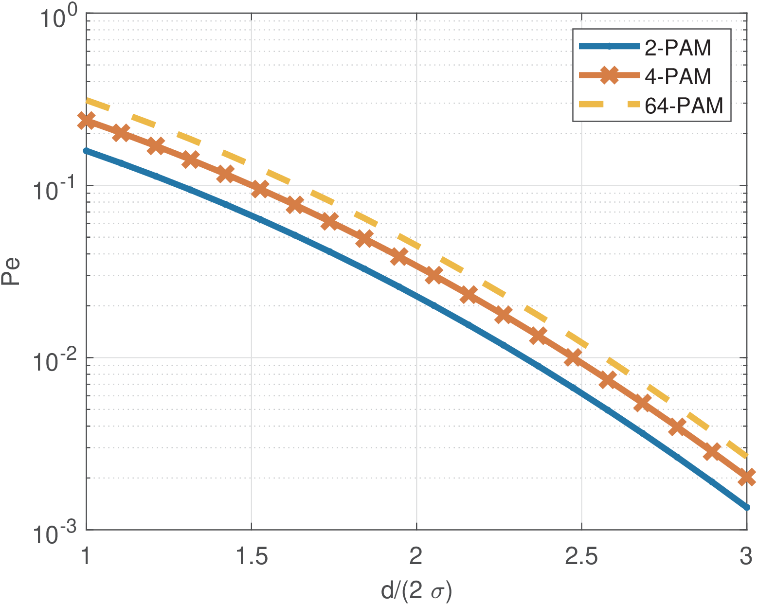
Figure 5.11: Comparison of $P_{e}$ obtained with three PAM systems as a function of $d∕(2σ)$ .

It is possible to compare different PAM systems using Eq. (5.6). Figure 5.11 informs $P_{e}$ for PAMs with $M = 2,4$ and 64. For a given $d∕(2σ)$ , $P_{e}$ is larger when $M$ increases.

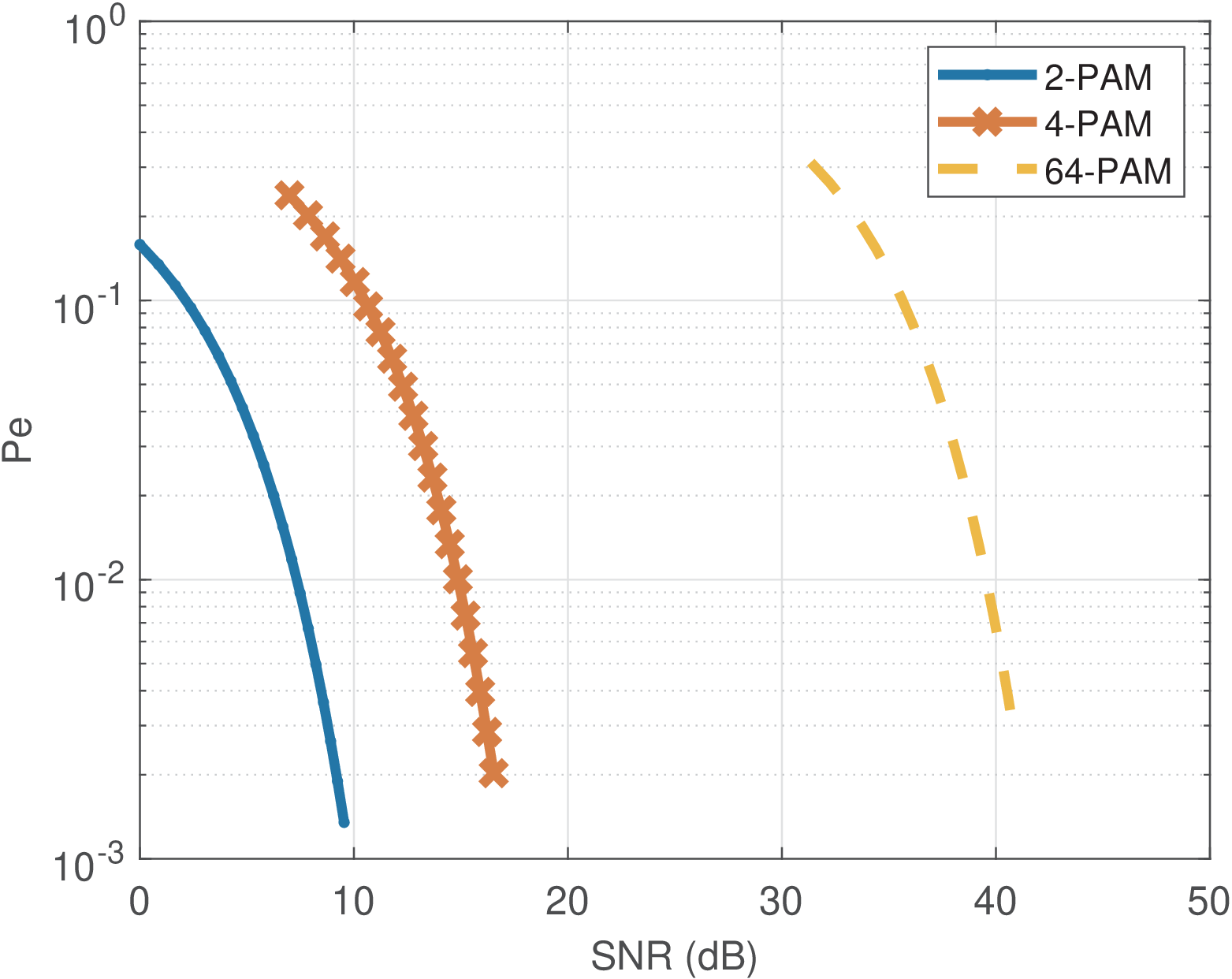
Figure 5.12: Comparison of $P_{e}$ obtained with three PAM systems as a function of the SNR (in dB) for the corresponding values of $d∕(2σ)$ in Figure 5.11.

Note that, when $d∕(2σ)$ is the same for different $M$ , the transmitted power increases with $M$ because the constellation expands while the distances $d$ between neighboring symbols is held fixed. This implies that, for a given $P_{e}$ , a larger SNR is required when $M$ increases. This fact is illustrated in Figure 5.12, which is a modified version of Figure 5.11 that uses the SNR in the abscissa. For example, to obtain $P_{e} = 0.01$ the 2-PAM, 4-PAM and 64-PAM require approximately 7, 15 and 40 dB of SNR, respectively.

One should be careful when using graphs as Figure 5.12 to compare distinct modulation schemes. There are important figures of merit in digital communications that are not taken into account in Figure 5.12 such as the bit rate $R$ and required bandwidth BW. Therefore, it is convenient to normalize the SNR as follows:

SNR = \frac{P_{s}}{P_{n}} = \frac{E_{s} ∕ T_{sym}}{2 BW \frac{N_{0}}{2}} = \frac{E_{b} b R_{sym}}{BW N_{0}} = \frac{E_{b}}{N_{0}} \frac{R}{BW},

which is equivalent to

\frac{E_{b}}{N_{0}} = SNR \frac{BW}{R} .

(5.14)

For example, assuming $R = 40$ kbps and $BW = 80$ kHz, an $E_{b} ∕ N_{0} = 14$ dB in linear scale is approximately 25.12 and corresponds to an $SNR = 25.12(40∕80) = 12.56$ , which corresponds to approximately 11 dB.

Hence, the quantity $\frac{E_{b}}{N_{0}}$ can be interpreted as a normalized SNR. The BW in Eq. (5.14) is not (necessarily) the signal BW, but the BW at the receiver input.³ When using this equation, one may not use the BW of e. g. a shaping pulse (e. g., the value of $r$ when using raised cosines). In fact, in the case of discrete-time signals, $BW = F_{s} ∕2$ , which corresponds to the whole bandwidth. When performing a symbol-based simulation, $F_{s} = R_{sym}$ , such that

\frac{E_{b}}{N_{0}} = SNR \frac{BW}{R} = SNR \frac{F_{s} ∕2}{F_{s} b} = \frac{SNR}{2b}

(5.15)

or, equivalently, $SNR = 2b \frac{E_{b}}{N_{0}}$ .

For example, for a polar binary PAM signal with symbols ${−A,A}$ ( $d = 2A$ ) and assuming the shaping pulse has unitary energy, i. e., $⟨p(t),p(t)⟩ = 1$ , then $E_{b} = A^{2}$ . With the AWGN variance $σ^{2} = N_{0} ∕2$ and using Eq. (5.9), $P_{e}$ can be written as

P_{e} = Q (\frac{d}{2σ}) = Q (\sqrt{SNR}) = Q (\sqrt{\frac{2 E_{b}}{N_{0}}}) .

Note that, in this case ( $b = 1$ ), $SNR = \frac{2 E_{b}}{N_{0}}$ as indicated by Eq. (5.15).

It is useful to observe that $E_{b}$ can be estimated as the total energy $E_{t}$ of a signal divided by the number $N_{b}$ of bits in the signal. Assuming $E_{t}$ is the equivalent energy in Joules of a discrete-time signal $x[n]$ with $S$ samples, Eq. (E.21) and $N_{b} = R S T_{s}$ leads to

E_{b} = \frac{E_{t}}{N_{b}} = \frac{T_{s} ∑_{n=0}^{S−1} x^{2} [n]}{R S T_{s}} = \frac{E_{d}}{R S} = \frac{P_{c}}{R},

where $P_{c} = E_{d} ∕S$ is the equivalent signal power in Watts (see Section C.12.5).

For discrete-time signals sampled at $F_{s}$ , recall that the filtered WGN has variance

σ^{2} = 2 \frac{N_{0}}{2} BW = \frac{N_{0} F_{s}}{2}

because $BW = F_{s} ∕2$ .

Figure 5.13: Comparison of simulated and theoretical BER for binary PAM or BPSK using $E_{b} ∕ N_{0}$ . It should be compared to Figure 5.10.

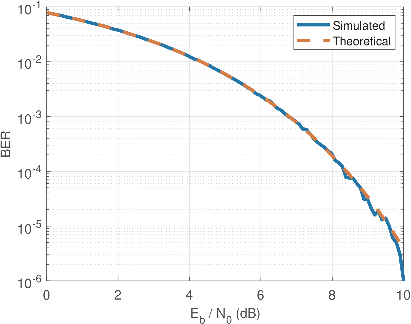
Figure 5.13 was generated with code Listing 5.4, which uses $E_{b} ∕ N_{0}$ and is similar to Listing 5.3, which uses SNR. When both $SNR$ and $E_{b} ∕ N_{0}$ are in dB, the difference is 3 dB as indicated by Eq. (5.15). Listing 5.4 adopted a larger number of transmitted bits because $P_{e}$ achieved values smaller than $1 0^{−5}$ .

Listing 5.4: MatlabOctaveBookExamples/ex_pam_ber_ebn0.m

1%Perform a symbol-based simulation for binary PAM / PSK 
2d=20; %Distance between symbols 
3A=d/2; %Amplitude A=d/2 Volts 
4R = 200; %rate in bps 
5Fs = R; %sampling rate in Hz 
6Nbits = 1e6; %Number of transmitted bits 
7bits = rand(1,Nbits)>0.5; %bits (0 or 1) 
8symbols = A*2*(bits-0.5); %symbols (-A or A) 
9ebN0_dB = linspace(0,10,100); %Eb/N0 in dB 
10ebN0 = 10 .^ (0.1*ebN0_dB); %linear Eb/N0 
11Eb = A^2/R; %energy per bit, or Eb=mean(symbols.^2)/R 
12N0 = Eb ./ ebN0; %one-sided AWGN PSD 
13noisePower = N0*Fs/2; %noise power (sigma^2) 
14V=length(noisePower); %number of points in grid 
15ber = zeros(1,V); %pre-allocate space 
16for i=1:V 
17    %generate noise 
18    noise = sqrt(noisePower(i)) * randn(size(symbols)); 
19    receivedSymbols = symbols + noise; %AWGN 
20    %recover bits using ML threshold equal to 0 
21    decodedBits = receivedSymbols > 0; 
22    ber(i) = sum(decodedBits ~= bits)/Nbits; %estimate BER 
23end 
24%compare with theoretical expression: 
25theoreticalBER = ak_qfunc(sqrt(2*ebN0)); 
26clf,semilogy(ebN0_dB,ber,ebN0_dB,theoreticalBER,'--'); 
27xlabel('E_b / N_0 (dB)'); ylabel('BER'); grid; 
28legend('Simulated','Theoretical');

Listing 5.5 compares the Monte Carlo simulation of 16-QAM with the theoretical expression for $P_{e}$ .

Listing 5.5: MatlabOctaveBookExamples/ex_qam_ber.m

1%Perform a symbol-based simulation for square M-QAM 
2M=16; 
3snr_dB = linspace(0,16,100); %SNR in dB 
4const=ak_qamSquareConstellation(M); %constellation 
5Nsymbols=1e7; %number of symbols 
6txIndices = floor(M*rand(1,Nsymbols)); %0 to M-1 
7symbols = const(txIndices+1); %transmitted symbols 
8snr = 10 .^ (0.1*snr_dB); %linear SNR 
9signalPower = mean(abs(symbols).^2); %must use abs() 
10%noisePower is the noise power "per dimension". For QAM 
11%N=2 dimensions and the total noise power is 2*noisePower 
12noisePower=(signalPower ./ snr)/2; %noise power (sigma^2) 
13V=length(noisePower); %number of points in grid 
14ser = zeros(1,V); %pre-allocate space 
15for i=1:V 
16    %complex noise 
17    noise = sqrt(noisePower(i)) * randn(size(symbols))+... 
18        j * sqrt(noisePower(i)) * randn(size(symbols)); 
19    receivedSymbols = symbols + noise; %AWGN 
20    decodedSymbolIndices=ak_qamdemod(receivedSymbols,M); 
21     %estimate SER 
22    ser(i)=sum(decodedSymbolIndices~=txIndices)/Nsymbols; 
23end 
24%compare with theoretical expression: 
25qvalues = ak_qfunc(sqrt(3*snr/(M-1))); 
26temp = (1-1/sqrt(M))*qvalues; 
27theoreticalSER = 4*(temp  - temp.^2); 
28clf, semilogy(snr_dB,ser,snr_dB,theoreticalSER,'--'); 
29xlabel('SNR (dB)'); ylabel('SER'); grid; 
30legend('Simulated','Theoretical');

Listing 5.6 consists of a version of Listing 5.5 using $E_{b} ∕ N_{0}$ instead of SNR. Note that for consistency, the SNR range used in both was the same.

Listing 5.6: MatlabOctaveBookExamples/ex_qam_ber_ebn0.m

1%Perform a symbol-based simulation for square M-QAM 
2M=16; %number of symbols 
3ebN0_dB = linspace(0,14,20); %SNR in dB 
4Nsymbols=1e5; %number of symbols 
5b=log2(M); %number of bits per symbol 
6const=ak_qamSquareConstellation(M); %constellation 
7Rsym = 400; %symbol rate (bauds) 
8R = Rsym*b; %rate in bps 
9Fs = Rsym; %sampling rate in Hz 
10Nbits = Nsymbols*log2(M); %Number of transmitted bits 
11txIndices = floor(M*rand(1,Nsymbols)); %0 to M-1 
12symbols = const(txIndices+1); 
13ebN0 = 10 .^ (0.1*ebN0_dB); %linear Eb/N0 
14snr = ebN0 * R / Fs; %linear SNR 
15Eb=mean(abs(symbols).^2)/R; %energy per bit, note abs(.) 
16N0 = Eb ./ ebN0; %one-sided AWGN PSD 
17%noisePower is the noise power "per dimension". For QAM 
18%N=2 dimensions and the total noise power is 2*noisePower 
19noisePower = (N0*Fs)/2; %noise power (sigma^2) 
20V=length(noisePower); %number of points in grid 
21ser = zeros(1,V); %pre-allocate space 
22for i=1:V 
23    %generate complex noise 
24    noise = sqrt(noisePower(i)) * randn(size(symbols))+... 
25        j * sqrt(noisePower(i)) * randn(size(symbols)); 
26    %AWGN 
27    receivedSymbols = symbols + noise; 
28    decodedSymbolIndices=ak_qamdemod(receivedSymbols,M); 
29     %estimate SER 
30    ser(i)=sum(decodedSymbolIndices~=txIndices)/Nsymbols; 
31end 
32%compare with theoretical expression: 
33qvalues = ak_qfunc(sqrt(3*snr/(M-1))); 
34temp = (1-1/sqrt(M))*qvalues; 
35theoreticalSER = 4*(temp  - temp.^2); 
36clf,semilogy(ebN0_dB,ser,'x',ebN0_dB,theoreticalSER,'--'); 
37xlabel('E_b / N_0 (dB)'); ylabel('SER'); grid; 
38 
39%using Matlab: 
40[berm, serm] = berawgn(ebN0_dB, 'QAM', M); 
41hold on 
42semilogy(ebN0_dB,serm,'or'); 
43 
44legend('Simulated','Theoretical','Matlab theo');

Figure 5.14: Comparison of M-QAM, M-PSK and the Shannon limit.

Instead of using $P_{e}$ , it is sometimes more interesting to use $P_{b}$ for comparing different modulation schemes. Because analytically calculating $P_{b}$ is sometimes unfeasible, it is commonly assumed that Gray coding is used and $P_{b} = P_{e} ∕b$ , i. e., each symbol error leads to only one bit error. Under this assumption, the following two approximations can be used:

P_{b}^{QAM} ≈ \frac{4}{b} (1 − \frac{1}{\sqrt{M}}) Q (\sqrt{\frac{3b E_{b} ∕ N_{0}}{M − 1}})

and

P_{b}^{PSK} ≈ \frac{2}{b} Q (\sqrt{\frac{2b E_{b}}{N_{0}}} sin (\frac{π}{M})),

for M-QAM and M-PSK, respectively. These expressions inform the amount of power required to reach a given $P_{b}$ . It is useful to use the spectral efficiency and observe the bandwidth requirement. For a QAM

η_{max}^{QAM} = \frac{R_{sym} b}{BW} = b.

(5.16)

because a QAM over a (bandpass) channel of bandwidth $BW$ , can use $R_{sym} = BW$ for zero ISI when assuming zero excess bandwidth.

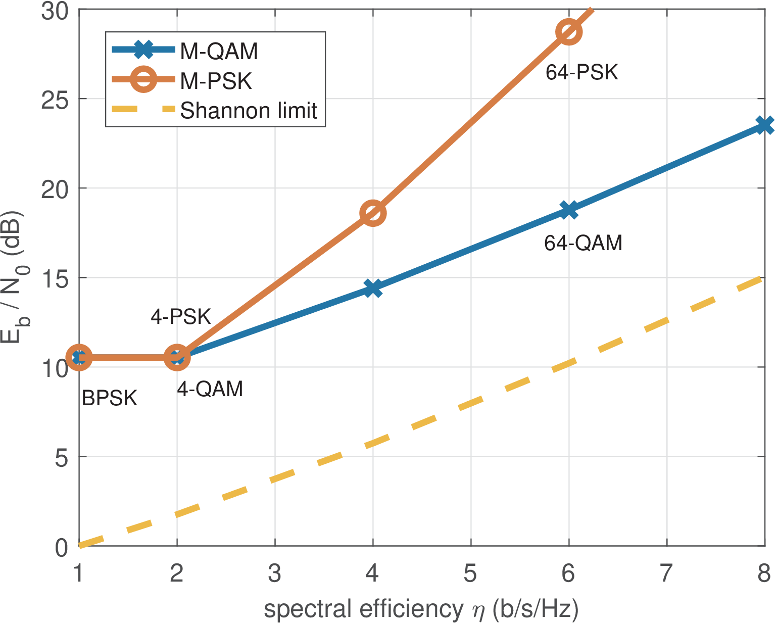
Hence, using Eq. (5.16), which is also valid for M-PSK, Listing 5.7 makes this comparison, which results in Figure 5.14.

Listing 5.7: MatlabOctaveCodeSnippets/snip_digi_comm_modulation_compare.m

1Pb=1e-6; %target bit error probability 
2b=2:2:8; %range of bits per symbol 
3M=2.^b; %number of symbols 
4qarg = Pb*b./(4*(1-1./sqrt(M))); %argument of Q^{-1} 
5gap = 1/3 * ak_qfuncinv(qarg).^2; %gap to capacity 
6EbN0_qam = gap .* (2.^b -1) ./ b; %for QAM 
7EbN0_psk = (ak_qfuncinv(qarg).^2)./(2*b.*(sin(pi./M)).^2); 
8EbN0_qam_dB = 10*log10(EbN0_qam); %in dB 
9EbN0_psk_dB = 10*log10(EbN0_psk); %in dB 
10EbN0_binary = 10*log10((ak_qfuncinv(Pb)^2)/2); %for BPSK 
11b=[1 b]; %pre-append the result for BPSK (or binary PAM) 
12EbN0_psk_dB = [EbN0_binary EbN0_psk_dB]; 
13EbN0_qam_dB = [EbN0_binary EbN0_qam_dB]; 
14EbN0_shannon_dB = 10*log10((2.^b -1) ./ b); %Shannon limit 
15plot(b,EbN0_qam_dB,b,EbN0_psk_dB,b,EbN0_shannon_dB);

Figure 5.14 shows that, as the spectral efficiency increases, the gap between the PSK performance and the Shannon limit becomes larger. In contrast, this gap remains approximately constant for QAM. When $η = 2$ and 8, the QAM gaps are approximately 8.77 and 8.48 dB, respectively.

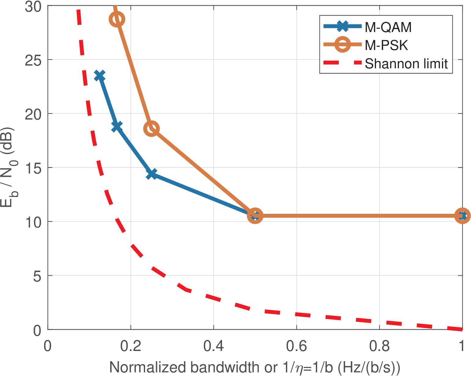
Figure 5.15: An alternative comparison of M-QAM, M-PSK and the Shannon limit, which contains the same information as Figure 5.14.

Figure 5.15 is an alternative to Figure 5.14 in which the abscissa is $1∕η$ instead of $η$ . The value $1∕η$ can be interpreted as a normalized bandwidth $BW ∕R$ , which is $1∕b$ in this case. Figure 5.15 illustrates the tradeoff between transmitted power and bandwidth. For a given $P_{b}$ , when $b$ increases, less bandwidth is required at the expense of a larger signal power.

³ See the discussion at [ url5ebn].