MAP and ML Receivers for Symbol-by-Symbol Decisions

5.3 MAP and ML Receivers for Symbol-by-Symbol Decisions

This section discusses two decision criteria widely adopted in communication receivers: maximum a posteriori (MAP) and maximum likelihood (ML). Under some conditions, MAP and ML can be the optimum data detection strategy for minimizing $P_{e}$ . For example, for the AWGN channel, MAP executed in a symbol-by-symbol basis (in this case the channel is memoryless) is the optimum criterion. When the symbols are uniformly distributed, ML is equivalent to MAP and, consequently, ML is optimum for AWGN with uniform symbol priors.

The discussion assumes the receiver knows all $M$ conditional PDFs $p(r|m)$ and they are the correct ones. MAP and ML also guide the receiver in the situation where a decision must be done of a sequence of symbols. But here, for simplicity, only symbol-by-symbol decisions are discussed.

When using the ML criterion, the receiver defines the decision regions by choosing:

{\hat{m}}_{}

ML =

arg max_{m_{i}} p(r| m_{i}).

Hence, after observing a given value

r = R

, all values

p(r = R| m_{i})

for the symbols

m_{i}

i = 1,…,M

, are calculated and the chosen symbol is the one that achieves the maximum

p(r = R| m_{i})

Note that, commonly, the elements of $r$ are continuous random variables. For example, for AWGN, $r$ is distributed according to a Gaussian. Hence, $p(r = R|m)$ is not a probability but a likelihood (in the context of this text, the value of a continuous PDF or the PDF itself). This is the reason for the name ML criterion. ML does not take into account the prior probabilities $p(m)$ , which can be important, as illustrated by the example in Figure 5.4.

The distinction with respect to ML is that MAP takes the priors in account and is the optimum solution in the general case of non-uniform priors.

The MAP criterion seeks the maximization of the posteriori distribution $p(m|r)$ :

{\hat{m}}_{}

MAP =

arg max_{m_{i}} p(m_{i} |r). (5.2)

The posteriors

p(m_{i} |r)

can be obtained via the Bayes’ theorem as in Eq. (A.62), repeated here for convenience:

p(m_{i} |r) = \frac{p(r| m_{i})p(m_{i})}{p(r)} = \frac{p(r| m_{i})p(m_{i})}{∑_{j=1}^{M} p(m_{j})p(r| m_{j})} .

Because $p(r)$ is the same normalization factor for all candidates $m_{i}$ , Eq. (5.3) is equivalent to

{\hat{m}}_{}

MAP =

arg max_{m_{i}} p(r| m_{i})p(m_{i}). (5.3)

Eq. (5.3) should be compared to Eq. (5.1). It is possible to prove that the decision regions imposed by the MAP criterion are optimal according to the following reasoning, which assumes

r

is a discrete r. v. for simplicity.²

For each received $r$ , if there is only one symbol $m_{i}$ for which $p(r| m_{i}) > 0$ , then $\hat{m} = m_{i}$ and $r$ does not contribute to $P_{e}$ . If there are two or more symbols $m_{i}$ for which $p(r| m_{i}) > 0$ , then the decision will surely influence $P_{e}$ . In order to see that, assume the symbols for which $p(r| m_{i}) > 0$ are $m_{1}, m_{2}$ and $m_{3}$ . Choosing $m_{1}$ would imply adding the parcels $p(r| m_{2})p(m_{2}) + p(r| m_{3})p(m_{3})$ to $P_{e}$ (see Eq. (5.1)), while choosing $m_{2}$ would imply adding the parcels $p(r| m_{1})p(m_{1}) + p(r| m_{3})p(m_{3})$ . Therefore, choosing $\hat{m} = arg max_{m∈ M} p(r|m)p(m)$ is the optimal decision because it minimizes the parcel that contributes to $P_{e}$ .

As mentioned, when the symbols are uniformly distributed, i. e., all priors $p(m) = 1∕M$ are the same, the ML and MAP criteria lead to the same result. For AWGN, all $p(r|m)$ are Gaussians with the same variance (imposed by the noise) and the symmetry derived from uniform priors reflects in having thresholds that are the same for ML and MAP and in the middle point between neighbor symbols. Figure 5.5 provides an example, where the ML thresholds are relatively easy to obtain as $− 2,0,2$ by observation when the likelihood PDFs cross each other.

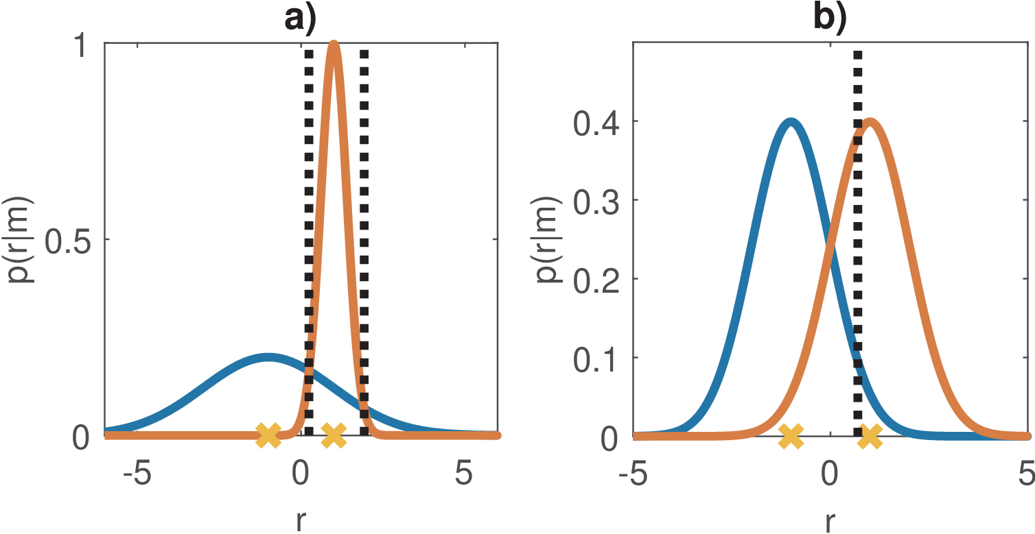
Figure 5.6: Conditional probabilities $p(r|m)$ and MAP thresholds. In case a) the priors are uniform but the variances of the noises added to each symbol differ while in b) the variances are the same (as in AWGN) but the priors differ.

To get insight, a more general case is assumed in the sequel. Assume binary modulation with symbols $m_{1}$ and $m_{2}$ , where $p(r| m_{1}) = N(r| μ_{1}, σ_{1})$ and $p(r| m_{2}) = N(r| μ_{2}, σ_{2})$ with $σ_{1} ≠ σ_{2}$ . The goal is to calculate the values of $r$ for which $p(m_{1})p(r| m_{1}) = p(m_{2})p(r| m_{2})$ because they correspond to the threshold of the MAP decision regions:

\begin{array}{l} p(m_{1}) \frac{1}{\sqrt{2π} σ_{1}} e^{− \frac{{(r− μ_{1})}^{2}}{2 σ_{1}^{2}}} & = p(m_{2}) \frac{1}{\sqrt{2π} σ_{2}} e^{− \frac{{(r− μ_{2})}^{2}}{2 σ_{2}^{2}}} \\ ln (\frac{p(m_{1}) σ_{2}}{p(m_{2}) σ_{1}}) & = \frac{{(r − μ_{1})}^{2}}{2 σ_{1}^{2}} − \frac{{(r − μ_{2})}^{2}}{2 σ_{2}^{2}} \end{array}

This is a second order equation $a r^{2} + br + c = 0$ and the two thresholds are $r = \frac{−b± \sqrt{b^{2} −4ac}}{2a}$ , where $a = σ_{2}^{2} − σ_{1}^{2}$ , $b = 2(σ_{1}^{2} μ_{2} − σ_{2}^{2} μ_{1})$ and $c = σ_{2}^{2} μ_{1}^{2} − σ_{1}^{2} μ_{2}^{2} − 2 σ_{1}^{2} σ_{2}^{2} ln ((σ_{2} p(m_{1}))∕(σ_{1} p(m_{2})))$ .

Figure 5.6 was generated with the code ak_MAPforTwoGaussians.m that implements this calculation. In case a), the priors are uniform but the variances (2 and 0.4) are distinct and $p(r| m_{1}) = N(r|− 1,2)$ , $p(r| m_{2}) = N(r|1,0.4)$ , as if the noise had distinctly affected the two symbols. Then, there are two thresholds of interest, which is always the case when $σ_{1}^{2} ≠ σ_{2}^{2}$ . The MAP optimal thresholds are 0.24 and 1.93, which coincide with the ML thresholds. A receiver that uses these two thresholds to make its decisions would achieve the Bayes error (the minimum $P_{e}$ ), which in this case is $P_{e} = 0.117$ . In case b), the variances are the same such that $p(r| m_{1}) = N(r|− 1,1)$ and $p(r| m_{2}) = N(r|1,1)$ , but the threshold is not in the middle point because the priors $p(m_{1}) = 0.8$ , $p(m_{2}) = 0.2$ differ. In this case, because $m = 1$ has larger prior probability $p(m_{1}) = 0.8$ , the MAP optimal threshold is 0.69 and is biased in favor of the symbol $m_{1}$ .

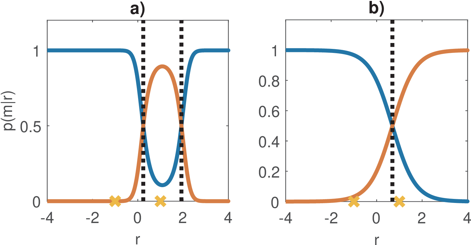
Figure 5.7: Posteriori distributions $p(m|r)$ for the examples in Figure 5.6. Note that while $p(r|m)$ are likelihoods, $p(m|r)$ are probabilities and sum up to one.

Figure 5.7 shows the posteriori distributions $p(m|r)$ for the examples in Figure 5.6. While the MAP threshold for case b) in Figure 5.6 cannot be found visually, it is very easy to note that 0.69 is the optimal threshold via Figure 5.7.

It should be noted that for AWGN, because the Gaussian distribution is such that the distance to the mean is inversely proportion to the probability, the thresholds obtained for the ML criterion coincide with the threshold of Voronoi regions defined by the Euclidean distances among the symbols.

² It is also assumed that $p(m) > 0,∀m$ , otherwise the effective number of symbols would be less than $M$ .