Applications

2.14 Applications

Application 2.1. Signal regeneration: Analog versus digital communications This application illustrates the idea of signal regeneration in digital communication systems. Assume the information is conveyed by the signal amplitude. Because a finite set of amplitudes is used by the transmitter, small variations on the received signal amplitudes can be identified and corrected. Assume an original digital signal $x_{q} [n]$ , with $M = {- 2, - 1, 0, 1, 2}$ , is contaminated by additive noise $n [n]$ , and a new signal $z [n] = x_{q} [n] + n [n]$ is created. This noise contamination can happen when transmitting a signal in telecommunication or copying a CD, for example. If the magnitude $| n [n] |$ is not too large (in this case, $| n [n] | < 0.5$ ), it is possible to successfully recover $x_{q} [n]$ by approximating the samples of $z [n]$ to the nearest value in $M$ .

Figure 2.28: Example of successful regeneration of a digital signal at $SNR = 3$ dB. The top-left plot is the transmitted signal $x_{q} [n]$ , the top-right is the noise $n [n]$ , the bottom-left is the regenerated signal $y_{q} [n]$ and the bottom-right is the error $y_{q} [n] - x_{q} [n]$ .

Figure 2.29: Example of unsuccessful regeneration of a digital signal at $SNR = - 3$ dB. Three errors can be observed at $n = 3, 6$ and 8.

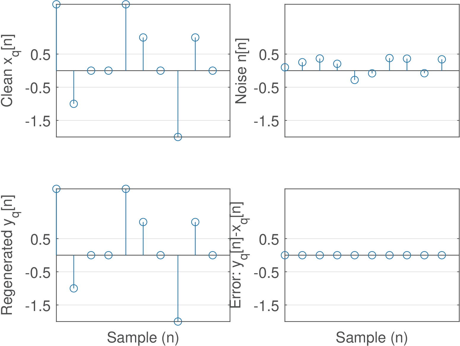
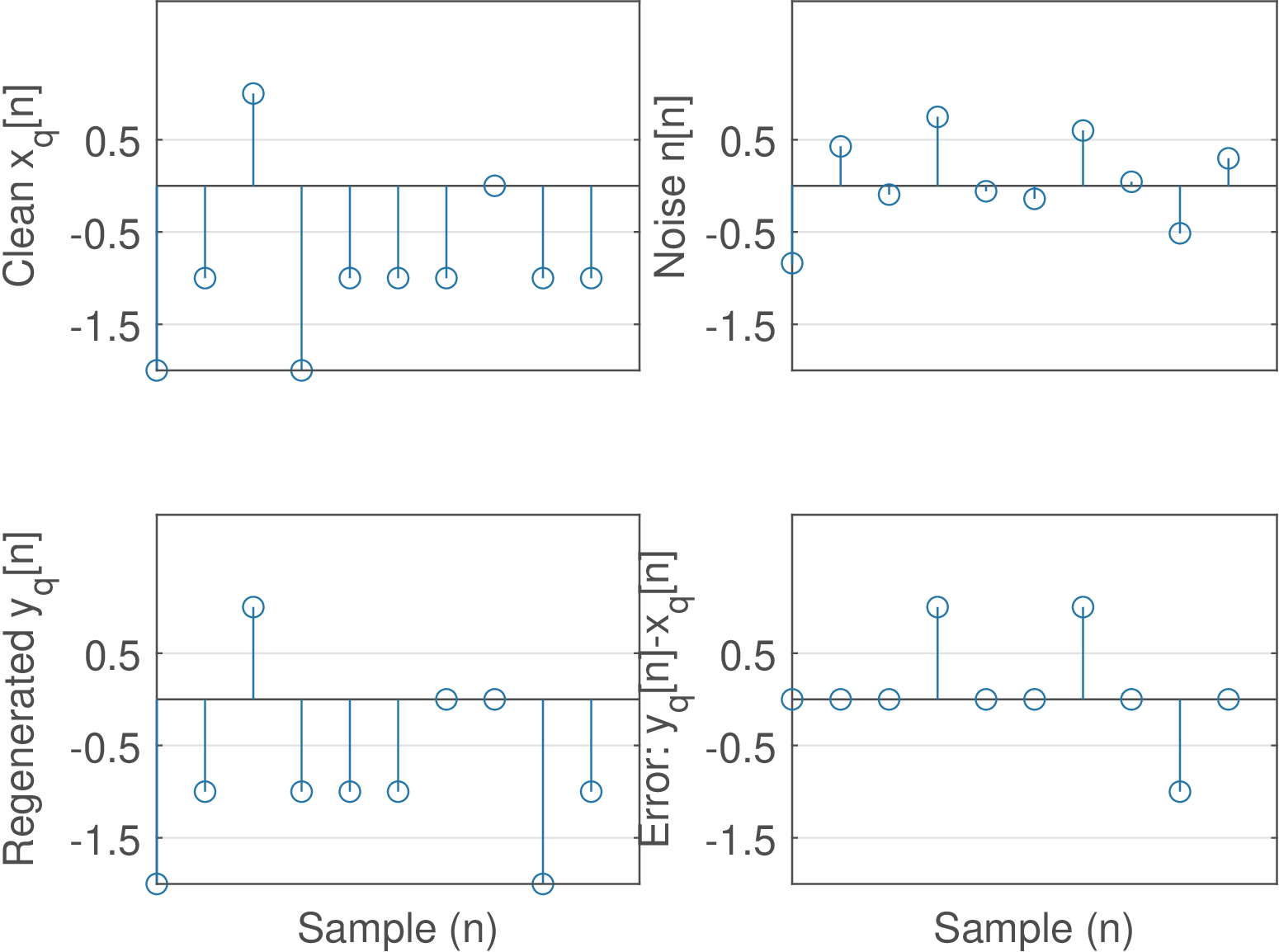
Figure 2.28 depicts samples of these signals in the case that the signal-to-noise ratio (SNR) is 3 decibels (dB), i. e., the power of $x_{q} [n]$ is approximately twice the power of $n [n]$ (see Appendix A.27 for an explanation about the decibel). In this case, $x_{q} [n]$ was recovered without errors. To complement the example, Figure 2.29 was generated at similar conditions but with SNR $= - 3$ dB. Note $| n [n] | > 0.5$ for $n = 0, 3, 6, 8$ but $x_{q} [0] = - 2$ could be recovered because $n [n]$ was negative and $- 2$ is the nearest value for all received amplitudes larger than $- 1.5$ . Hence, three errors were created in the process. $□$

Application 2.2. Packing the data into $b$ bits and vice-versa. Before discussing the transmission, it is important to consider an appropriate procedure to convert the input data into the required number of bits.

There are many possible implementations of such procedure. The companion code ak_sliceBytes.m and ak_unsliceBytes.m illustrate a simple implementation that assumes the information to be transmitted is originally organized in bytes. This is a sensible assumption given that most programming languages provide support to reading and writing bytes from/to files and networks.

The implemented function has, as input argument, the number $b$ of bits per symbol. The task is to convert each byte (0 to 255 in decimal) to chunks of $b$ bits each. Hence, each chunk corresponds to a number in the range $[0, 2^{b} - 1]$ in decimal. For example, the command

1inputBytes = [4, 255, 22]; b=4; 
2chunks = ak_sliceBytes(inputBytes, b)

outputs chunks =[0 4 15 15 1 6]. Note that 3 bytes (24 bits) were properly split into 6 chunks of 4 bits each. The last byte, 22 in decimal, corresponds to 00010110 in binary. Hence, it is split into chunks 0001 and 0110 in binary or, equivalently, 1 and 6 in decimal. In all these manipulations, Matlab/Octave internally treats these values as integer numbers (and may use 64 bits to represent each number, either a “byte” or a “chunk”), but for the sake of digital communication simulations, the important aspect is the dynamic range of the number. The range indicates how many bits are necessary to represent that number. It should be noted that ak_sliceBytes.m has a simple implementation: it is very slow and limited to $b \in {1, 2, 4, 8}$ .

The function ak_unsliceBytes.m performs the inverse operation. The command

1outputBytes = ak_unsliceBytes(chunks, b)

recovers the bytes such that outputBytes=[4, 255, 22].

When dealing with sequences of 0’s and 1’s, the functions ak_sliceBitStream and ak_unsliceBitStream can be used. For example, the command ak_sliceBitStream([0 0 1 1 1 1], 3) (the second argument is the number of bits per symbol) outputs [1 7], while the command ak_unsliceBitStream([1 7], 3) recovers the bit stream. $□$

Application 2.3. Packing data into bits and vice-versa using GNU Radio.

In GNU Radio (GR), the bits are typically packed into integers that are called chunks. For example, taking Listing 2.6 as reference, the elements of symbolIndicesTx and symbolIndicesRx are the chunks. One distinction between Matlab/Octave and GR is that in the former the first array index is 1 while it is 0 in GR.

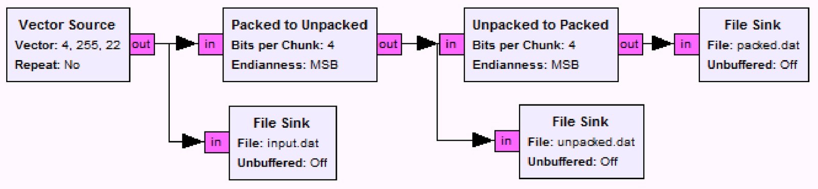
When using GR, the procedures discussed in Application 2.2 are performed by the blocks within the group ‘Misc Conversions’ named ‘Unpacked to Packed’ and ‘Packed to Unpacked’ (assuming GR version 3.6.2). The configuration of these blocks include the input data type (32-bits int, 16-bits short, byte), ordering convention (MSB or LSB) and number of input/output ports.

A simple setup is illustrated in Figure 2.30, with some File Sink blocks added for convenience to save the data (bytes, as binary files).

Figure 2.30: Example of un/pack operations in GNU Radio (from ak_unpack_pack.grc).

The generated files can be inspected using Python, for example:

1# reading file sink result 
2from numpy import * 
3input = list(fromfile(open('input.dat'), dtype=uint8)) 
4unpacked = list(fromfile(open('unpacked.dat'), dtype=uint8)) 
5packed = list(fromfile(open('packed.dat'), dtype=uint8))

where uint8 indicates the representation as bytes. This code generates the following output:

1>>> input 
2[4, 255, 22] 
3>>> unpacked 
4[0, 4, 15, 15, 1, 6] 
5>>> packed 
6[4, 255, 22]

with the output file packed.dat having the same contents of input.dat. Learning how to perform packing and unpacking is essential to understand GR. $□$

Application 2.4. Some code to estimate SER and BER. The function ak_calculateSymbolErrorRate.m listed in Listing 2.17 estimates the SER.

Listing 2.17: MatlabOctaveFunctions/ak_calculateSymbolErrorRate.m

1function ser=ak_calculateSymbolErrorRate(symIndicesTx,symIndicesRx) 
2% function ser=ak_calculateSymbolErrorRate(symIndicesTx,symIndicesRx) 
3%Get percentage of wrong symbols (sym) by comparing two sequences: 
4numErrors=sum(symIndicesTx ~= symIndicesRx); %number of errors 
5N=length(symIndicesTx); %N is the number of symbols 
6ser = numErrors / N; %estimated probability of an error

Similarly, the function ak_estimateBERFromBytes.m calculates the bit error probability (BER), or $P_{b}$ , between two sequences of bytes. For example, the command ber = ak_estimateBERFromBytes([0 254],[255 255]) informs ber = 0.5625, which correctly corresponds to 9 different bits out of 16, i. e., a BER of 56.25%. If the elements are restricted to values 0 or 1, the function ak_estimateBERFromBits.m can be used. The code ak_estimateBERFromBytes.m, for calculating the BER when the data is organized in bytes, is a little more involved and slower than the codes for calculating the SER and ak_estimateBERFromBits.m. $□$

Application 2.5. Transmitting the bytes of a file. Here the channel is assumed noise-free and with unlimited bandwidth. Therefore, it can transmit an infinite number of bits per second without errors. Listing 2.18 provides an example using $R_{sym} = F_{s} = 100$ Hz and $b = 4$ bits/symbol. The rate is $R = R_{sym} \times b = 400$ bps.

Listing 2.18: MatlabOctaveBookExamples/ex_pam_idealchannel.m

1fileHandler=fopen('myfile.bin','r'); %open in binary mode 
2if fileHandler==-1 %check if successful 
3    error('Error opening the Tx file! Does it exist?'); 
4end 
5inputBytes=fread(fileHandler, inf, 'uchar'); %read bytes 
6fclose(fileHandler); %close the input file 
7b=4; %number of bits per symbol 
8M=2^b; %number of symbols 
9constel = -(M-1):2:(M-1); %create PAM constellation 
10%Use oversampling L=1, such that symbol rate = Fs 
11Fs=100; %sampling frequency in Hz 
12chunksTx = ak_sliceBytes(inputBytes, b); %"cut" bytes 
13symbols = constel(chunksTx+1); %get the Tx symbols 
14s = symbols; %oversampling=1, send the symbols themselves 
15r = s; %ideal channel: received signal = transmitted 
16[chunksRx, r_hat]=ak_pamdemod(r,M); %PAM demodulation 
17BER = ak_estimateBERFromBytes(chunksTx,chunksRx) %get BER 
18recoveredBytes = ak_unsliceBytes(chunksRx, b); %get bytes 
19fileHandler=fopen('received.bin','w');%open in binary mode 
20if fileHandler==-1 %check if successful 
21    error('Error opening the Rx file! Does it exist?'); 
22end 
23fwrite(fileHandler, recoveredBytes, 'uchar'); %write file 
24fclose(fileHandler); %close the file with received bytes

A software such as Linux’s diff can be used to compare the transmitted and received files (for example, diff received.bin myfile.bin), which must be exactly the same.

Note that the sampling frequency $F_{s}$ was defined in Listing 2.18 but not effectively used. One could simply increase its value to $F_{s} = 10$ MHz, for example, to have $R = 40$ Mbps. The BER would still be zero. Similarly, $b$ could be increased without bounds but the ones imposed by implementation issues (ak_sliceBytes limits $b$ to 8). Therefore there are two degrees of freedom to achieve infinite high rates under this ideal channel. In the sequel, it will be seen that, roughly, band-limited channels restrict the maximum $R_{sym}$ while AWGN restricts the maximum $b$ for a given BER. $□$

Application 2.6. PAM transmission. Other chapters discuss more about how to use group delay, equalization and matched filtering. But before that, it is useful to try an almost complete PAM transmission system. Some concepts may not be clear at this point, but the scripts can be executed again after reading more about the theory.

Listing 2.19 is a complete simulation of a 8-PAM transmission with AWGN added at the receiver with an SNR of 50 dB. The channel is bandpass with a 800 Hz bandwidth (from 3 to 3.8 kHz) and the transmitted signal is upconverted to a carrier frequency of 3400 Hz. The symbol rate is $R_{sym} = 250$ bauds such that the bit rate is $R = {log}_{2} 8 \times 250 = 750$ bps. All these parameters can be changed to study their impact on the system.

Listing 2.19: ../Applications/PAMSimple/ak_pamSimple.m

1%PAM example: transmission using frequency upconversion 
2%%%%%%%%% Parameters to be changed / tuned %%%%%%%%% 
3M = 8; %number of constell. symbols, b=log2(M) bits/symbol 
4Fs = 20000; %sampling frequency, Hz 
5L = 80; %oversampling factor. Assumed to be an even number 
6S = 100; %number of symbols to be transmitted 
7channelNumber = 1; %choose the channel, from 0 to 3 (2 is hardest) 
8showPlots = 1; %if 1, some plots are shown 
9Nequ = 40; %order of equalizer filter 
10verify_ISI_atTx = 1; %verify or not ISI at transmitter 
11useCorrelationForSync=1; %use crosscorrelation for synchronism? 
12%%%%%%%%% Fixed parameters, no need to change %%%%%%%%% 
13Fc1 = 3000; %passband channel, lower passband frequency 
14Fc2 = 3800; %passband channel, uppper passband frequency 
15BW = Fc2 - Fc1; %approximate channel bandwidth 
16Fc = (Fc1 + BW/2); %carrier frequency (Hz) 
17wc = 2*pi*Fc / Fs; %convert from W in rad/s to w in rad 
18%make all channels minimum phase to simplify equalization 
19ak_getChannel; %invoke script to get the channel 
20B_channel = ak_forceStableMinimumPhase(B_channel,0.1); 
21h=impz(B_channel,A_channel,400); %h[n] with 400 samples 
22h_equalizer=impz(A_channel,B_channel,Nequ+1); %equalizer 
23p = transpose(fir1(L,(BW/20)/Fs)); %shaping pulse (FIR filter) design 
24%make sure the sample corresponding to cursor is 1 
25cursorIndex=round((length(p)+1)/2); %assumes length(p) is odd 
26delayInSamples = cursorIndex; %filter delay equals cursor 
27scalingFactor = 1/p(cursorIndex); %find scaling factor... 
28p = p * scalingFactor; %to make p(cursorIndex) = 1 
29%generate baseband PAM symbols and transmitted signal 
30constellat=-(M-1):2:M-1; %PAM constellation 
31ind=floor(M*rand(S,1)); %random indices from 0 to M-1 
32pamSymbols=transpose(constellat(ind+1)); %sequence of random symbols 
33x=zeros(S*L,1); %pre-allocate space 
34x(1:L:end)=pamSymbols; %complete upsampling operation 
35xp=conv(x,p); %PAM baseband signal 
36if verify_ISI_atTx == 1 %check ISI at the transmitter 
37    zz=xp(delayInSamples:L:end); 
38    disp(['Power of ISI at Tx (should be zero) = ' ... 
39        num2str(mean((zz(1:S)-pamSymbols).^2)) ' Watts']) 
40end 
41%Frequency upconversion: modulate baseband PAM to wc 
42filterOrder=transpose(0:length(xp)-1); %"time" axis, as column vector 
43carrier = cos(wc*filterOrder); %generate carrier at transmitter 
44s = xp .* carrier; %transmitted signal 
45%Process signal through the channel 
46z=conv(s,h); %note that z is longer than s 
47%estimate the channel delay within the passband: 
48%[groupDelay,f]=grpdelay(h,1,linspace(Fc1,Fc2,50),Fs)%wrong in Octave 
49%[groupDelay,w]=grpdelay(h,1,(2*pi/Fs)*linspace(Fc1,Fc2,50),2*pi); 
50[groupDelay,w]=grpdelay(h,1,500); 
51wminNdx=find(w >= (2*pi*Fc1)/Fs,1,'first'); %indices for passband 
52wmaxNdx=find(w <= (2*pi*Fc2)/Fs,1,'last'); 
53channelDelayInSamples=round(mean(groupDelay(wminNdx:wmaxNdx))); %mean 
54delayInSamples=delayInSamples+channelDelayInSamples; 
55%generate AWGN with desired power 
56SNRdB = 50; %desired signal to noise ratio in dB 
57SNR=10^(0.1*SNRdB); %SNR in linear scale 
58powerRxSignal = mean(abs(z).^2); %signal power at receiver 
59noisePower = powerRxSignal/SNR %noise power 
60r = z + sqrt(noisePower)*randn(size(z)); %add noise 
61r = conv(r,h_equalizer);%equalization (one can eventually disable it) 
62%command below did not work on Octave: 
63[groupDelay,f]=grpdelay(h_equalizer,1,linspace(Fc1,Fc2,50),Fs); 
64[groupDelay,w]=grpdelay(h_equalizer,1,500); %first, get for all range 
65wminNdx=find(w >= (2*pi*Fc1)/Fs,1,'first'); %indices for passband 
66wmaxNdx=find(w <= (2*pi*Fc2)/Fs,1,'last'); %now only for passband: 
67equalizerDelayInSamples=round(mean(groupDelay(wminNdx:wmaxNdx))) 
68delayInSamples = delayInSamples + equalizerDelayInSamples; 
69%regenerate carrier at the receiver 
70filterOrder=transpose(0:length(r)-1); %"time" axis, as column vector 
71carrier = cos(wc*filterOrder); %create carrier 
72r2 = r .* carrier; %r2 has images at DC and twice wc 
73%design receiver filter to eliminate images: 
74%Obs: on Matlab, firpmord allows to specify attenuation, e.g. 
75%lowpass filter of order n=292 (attenuation 0.01): 
76% [n,fo,mo,w]=firpmord([BW/3 BW/2],[1 0],[0.01 0.01],Fs); 
77%or lowpass of order n=489 (attenuation 0.001) at stopband: 
78% [n,fo,mo,w]=firpmord([BW/3 BW/2],[1 0],[0.001 0.001],Fs); 
79% p_rx = firpm(n,fo,mo,w); %then design the filter with given order 
80%Instead of firpm, use firls, supported by both Octave and Matlab 
81filterOrder=489; %filter order 
82p_rx = firls(filterOrder,[0 BW/Fs BW/Fs 1],[1 1 0 0]); %design filter 
83disp(['Receiver filter has order = ' num2str(filterOrder)]) 
84xphat = conv(r2,p_rx); %filter the received signal 
85delayInSamples=delayInSamples+round((length(p_rx)-1)/2); 
86if useCorrelationForSync==1 %use xcorr or estimated delay 
87    [R,lags]=xcorr(xp,xphat,10*delayInSamples); 
88    maxLag=find(abs(R)==max(abs(R)),1,'first'); 
89    firstSymSample = abs(lags(maxLag)) + round(L/2); 
90else %simply use estimated delay 
91    firstSymSample = delayInSamples; 
92end 
93pamSymbolsRx=xphat(firstSymSample:L:end); %extract symbols 
94pamSymbolsRx=pamSymbolsRx(1:S); %eliminate tail 
95%normalize the received constellation 
96txConstellationPower = mean(constellat.^2); 
97rxConstellationPower = mean(pamSymbolsRx.^2); 
98pamSymbolsRx = pamSymbolsRx * ... 
99    sqrt(txConstellationPower/rxConstellationPower); 
100[chunksRx,r_hat]=ak_pamdemod(pamSymbolsRx,M);%demodulation 
101SER = 100*sum(pamSymbols ~= r_hat)/S %estimate SER 
102symError=pamSymbols-pamSymbolsRx;%calculate signal error 
103SNRrx_before_detection = 10*log10(mean(pamSymbols.^2)/... 
104    mean(symError.^2)) %SNR before detection 
105symError = pamSymbols - r_hat; %after detection 
106SNRrx_after_detection = 10*log10(mean(pamSymbols.^2)/... 
107    mean(symError.^2)) 
108Rsym = Fs/L; %symbol rate (in bauds) 
109Rbps = Rsym * log2(M); %bit rate (in bps) 
110disp(['Rate = ' num2str(Rbps) ' bps']) %show rate 
111if (showPlots==1) figs_pamSimple; end %show plots

The variable channelNumber is used by the function ak_getChannel, which allows to choose among 4 channels. The companion script figs_pamSimple shows the transmitted (TX) and received (RX) PSDs, the channel frequency response and group delay, etc. The script uses a zero-forcing equalizer designed in line h_equalizer=impz(A_channel,B_channel,Nequ+1), which simply inverts the channel. This strategy is problematic if the channel is not minimum-phase because the zeros of the channel outside or on the unit circle will be poles of the equalizer that will make it unstable (see Application E.16). Because of that, the function ak_forceStableMinimumPhase is used to eventually modify the original channel and make it minimum-phase, which allows to use such simple equalization strategy. A more practical method is to force the equalizer to be stable, even if the channel is not minimum-phase.

There are several filtering stages and each one adds a delay to its input signal. The variable delayInSamples keeps track of the total delay (in samples) and allows to perform a simple timing recovery.

Using the original code (without modifications), it should be noticed that channelNumber=3, which corresponds to having a FIR filter as channel, leads to a symbol error rate (SER) of 0. However, channelNumber=2, which corresponds to using an elliptic IIR filter as channel, leads to a nonzero SER. The reason is that this receiver does not use matched filtering and its default synchronization relies on delayInSamples, which is a fragile timing recovery strategy when the group delay varies significantly in the signal bandwidth. In fact, realigning the demodulated and transmitted symbols by just one symbol using plot(r_hat(1:end-1)-pamSymbols(2:end)) leads to the desired zero SER. It helps to see the received constellation to realize that the problem was timing, because the received symbols were clustered around the transmitted symbols. And to find the lag to use to realign, the xcorr function can be used. However, the goal is always to have an algorithm running an automatic estimation and not rely on manual adjustments. A more accurate timing recovery, vastly used in practice, can be obtained with cross-correlation by setting useCorrelationForSync=1, which then uses the method discussed in Application C.13.

Note that the cross-correlation can be used in the symbol or sample-domain, i. e., using sequences at rate $R_{sym}$ or $F_{s}$ , respectively. It is more accurate to work with the samples at $F_{s}$ but more computationally complex. Listing 2.19 illustrates with [R,lags]=xcorr(xp,xphat,10*delayInSamples) a strategy that is commonly used in practice: restrict the cross-correlation calculation to a specific (the narrowest possible) range of lags, in this case 10*delayInSamples. $□$

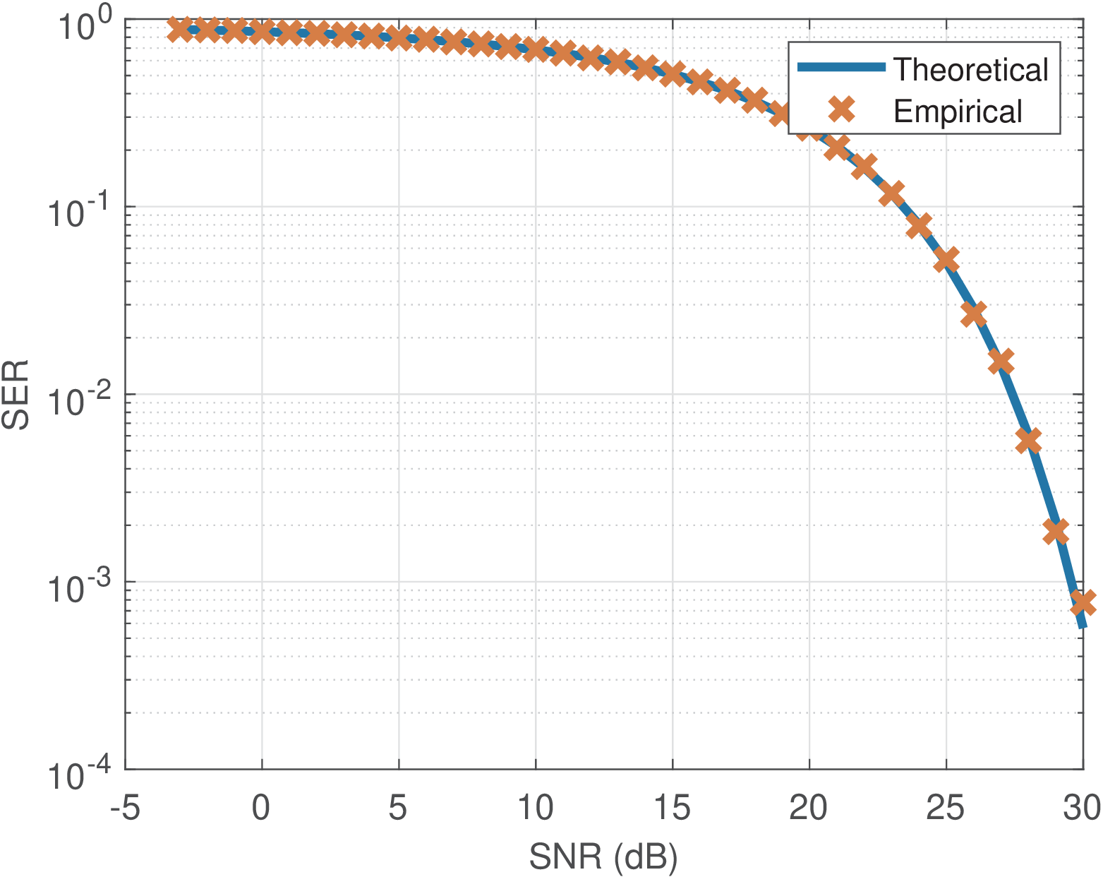
Application 2.7. Comparing theoretical SER with the ones obtained by symbol-based PAM simulation. Having the possibility of comparing to the theoretical SER is useful to validate implementations. To do that, it is necessary to generate signals with a given SNR. This can be done by properly scaling the signal or the noise. Most times it is not important which one is scaled. Listing 2.20 provides an example that scales the noise to obtain the SNRs of interest.

Listing 2.20: MatlabOctaveCodeSnippets/snip_digi_comm_theoretical_SER.m

1M=16; %modulation order 
2snrsdB=-3:30; %specified SNR range (in dB) 
3snrs=10.^(0.1*(snrsdB)); %conversion from dB to linear 
4numberOfSymbols = 40000; %number of symbols 
5alphabet = [-(M-1):2:M-1]; %symbols of a M-PAM 
6symbolIndicesTx = floor(M*rand(1, numberOfSymbols)); %randomly 
7s = alphabet( symbolIndicesTx +1); %transmitted signal 
8signalPower = mean(alphabet.^2); %signal power (Watts) 
9for i=1:length(snrs) %loop over all SNR of interest 
10    noisePower = signalPower/snrs(i); %noise power (Watts) 
11    n = sqrt(noisePower)*randn(size(s));%white Gaus. noise 
12    r = s + n; %add noise to the transmitted signal 
13    symbolIndicesRx = ak_pamdemod ( r, M); %decision 
14    SER_empirical(i) = sum(symbolIndicesTx ~= ... 
15        symbolIndicesRx)/numberOfSymbols%Symbol error rate 
16end 
17%Compare empirical and theoretical values of SER: 
18SER_theoretical=2*(1-1/M)*qfunc(sqrt(3*snrs/(M^2-1))); 
19semilogy(snrsdB,SER_theoretical,snrsdB,SER_empirical,'x');

Figure 2.31: Symbol error rate (SER) for distinct SNR values for 16-PAM.

The theoretical SER for PAM over AWGN is discussed later and given by Eq. (5.10), which is implemented with the command

1SER_theoretical=2*(1-1/M)*qfunc(sqrt(3*snrs/(M^2-1)));

in this case.

Figure 2.31 was generated with the previous code and shows a good match between the simulated (empirical) SER and its theoretical expression Eq. (5.10) for the given range of SNRs. These simulations are called Monte Carlo simulations and the empirical results sometimes are labeled Monte Carlo results. $□$

Application 2.8. Correspondences between convolution, correlation and inner product when using orthogonal expansions for transmission. The goal here is to understand how correlative decoding can be implemented in software. This can be achieved with cross-correlations, convolutions or even transforms.

Listing E.4 already demonstrated the correspondence between convolution and correlation. Now, Listing 2.21 shows an example where an inner product is obtained via a single value of a cross-correlation or a convolution.

Listing 2.21: MatlabOctaveCodeSnippets/snip_digi_comm_inner_product.m

1N=4; %length of vectors for inner product 
2x=(1:N)+j*(N:-1:1); %define some complex signals as row vectors, such 
3y=rand(1,N)+j*rand(1,N); %that fliplr inverts the ordering 
4innerProduct = sum(x.*conj(y)) 
5innerProductViaXcorr=xcorr(x,y,0) %cross-correlation at origin 
6innerProductViaConv=conv(x,conj(fliplr(y))); %use the second argument 
7innerProductViaConv=innerProductViaConv(N) %sample of interest

The inner products in Figure 2.26 can also be organized as a matrix multiplication. This gives a direct relation between the architecture of Figure 2.26 and a block transform. To illustrate that, Listing 2.22 uses matrices obtained via a Gram-Schmidt orthonormalization procedure to implement correlative decoding. Other transforms could be used, as long as the basis functions $φ_{i}$ of Figure 2.26 are properly mapped to the basis functions of the transform.

Listing 2.22: MatlabOctaveCodeSnippets/snip_digi_comm_correlative_decoding.m

1demodulationMethod='conv' %choose among: 'inner', 'xcorr' or 'conv' 
2SNRdB = 30; %AWGN SNR in dB 
3S=10000; %number of symbols to be generated 
4D=16; %space dimension, equivalent to oversampling factor 
5x=[ones(1,D) %define all possible transmit signal as row vectors 
6    -ones(1,D) 
7    ones(1,D/2) zeros(1,D/2) 
8    zeros(1,D/2) ones(1,D/2)]; 
9[M, temp] = size(x); %M is the number of input vectors, obs: temp = D 
10%M is also the modulation order (cardinality of the set of symbols) 
11[Ah,A]=ak_gram_schmidt(x,1e-12); %basis functions are columns of A 
12[N, temp] = size(Ah); %N is the number of basis functions (temp = D) 
13constellation=Ah*transpose(x); %find the constellation symbols 
14%% Transmitter 
15txIndices=floor(M*rand(1,S)); %random indices from [1, M] 
16m=constellation(:,txIndices+1); %obtain N random symbols 
17s=A*m; %obtain the signal to be transmitted (one column per symbol) 
18s=s(:); %concatenate all columns to create a one-dimensional signal 
19%% Channel 
20noise=sqrt(mean(abs(s).^2)/10^(0.1*SNRdB))*randn(S*D,1); %AWGN noise 
21r=s+noise; %add noise with specified SNR 
22rxSamples = reshape(r,D,S); %reorganize the samples as D x S matrix 
23%% Receiver 
24rxSymbols = zeros(N,S); %pre-allocate space 
25switch demodulationMethod %choose the demodulation "architecture" 
26    case 'inner' % Receiver via inner product (transform) 
27        rxSymbols = Ah*rxSamples; %symbols that represent signal 
28    case 'xcorr' % Receiver via cross-correlation 
29        for n=1:N %loop over all basis functions 
30            [R,lags]=xcorr(r,A(:,n)); %n-th basis function 
31            rxSymbols(n,:)=R(find(lags==0,1):D:end); %decimate 
32        end 
33    case 'conv' % Receiver via convolution 
34        for n=1:N %loop over all basis functions 
35            innerProductViaConv=conv(r,fliplr(A(:,n)'));%could use Ah 
36            rxSymbols(n,:)=innerProductViaConv(D:D:end); %decimate 
37        end 
38end 
39[rxIndices,m_hat]=ak_genericDemod(rxSymbols,constellation); %Decision 
40SER=sum(rxIndices ~= txIndices)/S %estimate the symbol error rate

Besides the transform-based implementation, Listing 2.22 also illustrates how a convolution and cross-correlation can be used for correlative decoding, providing the same result as an inner product. Choosing demodulationMethod in Listing 2.22, three distinct but equivalent (with respect to the output result) signal processing chains can be tested. For the suggested SNR of 30 dB, the system achieves a symbol error rate that is equal to zero.

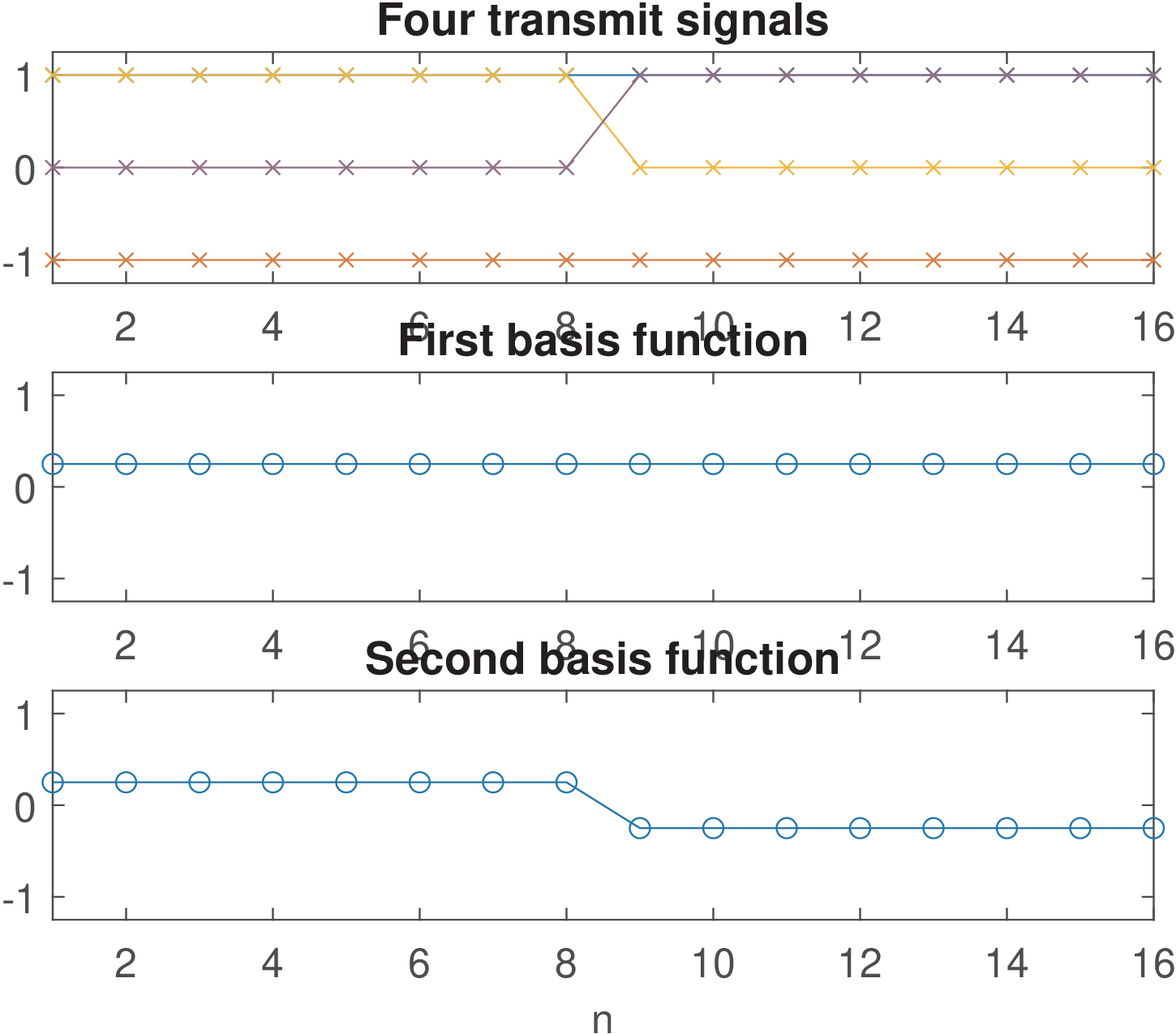
Figure 2.32: Gram-Schmidt inputs and outputs: four transmit signals and two corresponding basis functions.

In Listing 2.22, the $M = 4$ waveforms in matrix x can be represented by two basis functions derived by the Gram-Schmidt procedure. Figure 2.32 depicts both the waveforms in x (top plot) and the basis functions. The first waveform (row of x) is ones(1,D) and is the middle plot in Figure 2.32.

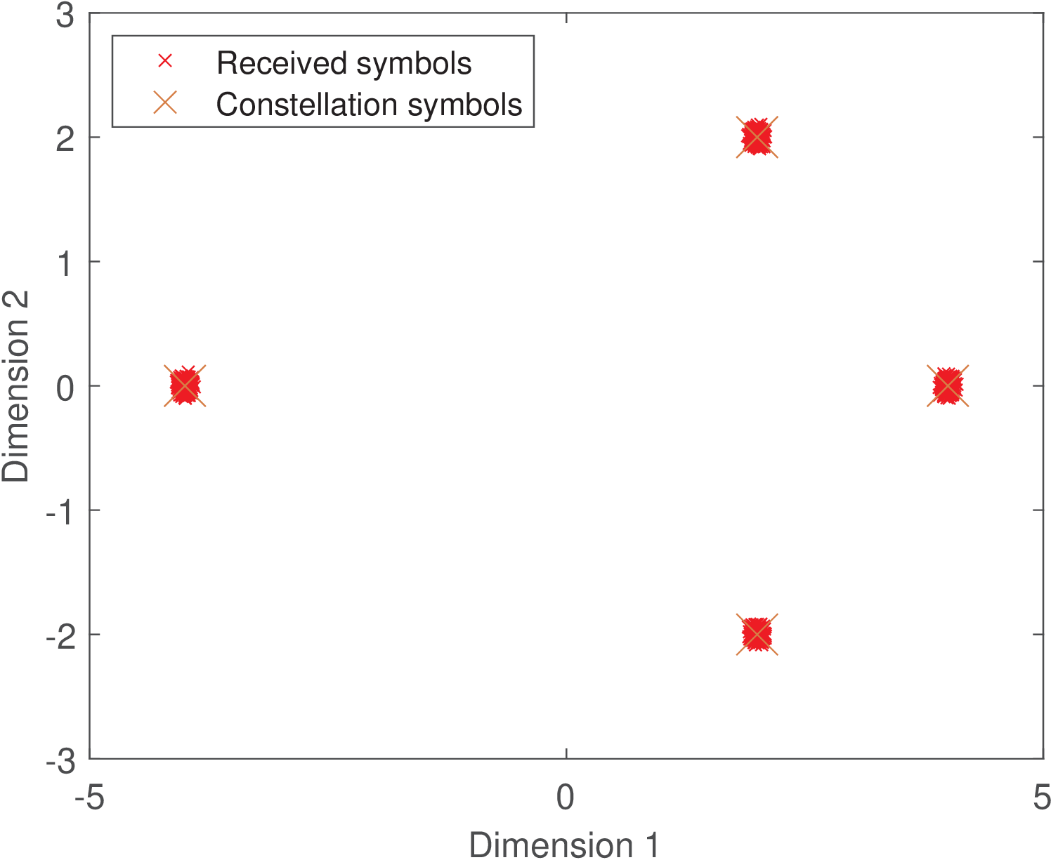
Figure 2.33: Constellation and received symbols ( $SNR = 30$ dB) of Listing 2.22.

Figure 2.33 shows the corresponding constellation with symbols $[4; 0]$ , $[- 4; 0]$ , $[2; 2]$ , $[2; - 2]$ . Because x was chosen just to provide a simple example, the resulting constellation is non-orthodox because it does not follow the guidelines discussed in Section 2.7.1 (in the context of PAM constellations). For example, its average is not at the origin!

Figure 2.34: Output samples for each basis functions and .

Using Figure 2.26 as reference, the basis functions $φ_{1}$ and $φ_{2}$ in Listing 2.22 are stored in A(:,1) and A(:,2), respectively. The received signal is processed using each basis functions, in parallel, as suggested by Figure 2.26. In case the method is ’xcorr’ or ’conv’, this parallel processing is explicit, but it is equivalent to the multiplication by the transform matrix in rxSymbols = Ah*rxSamples.

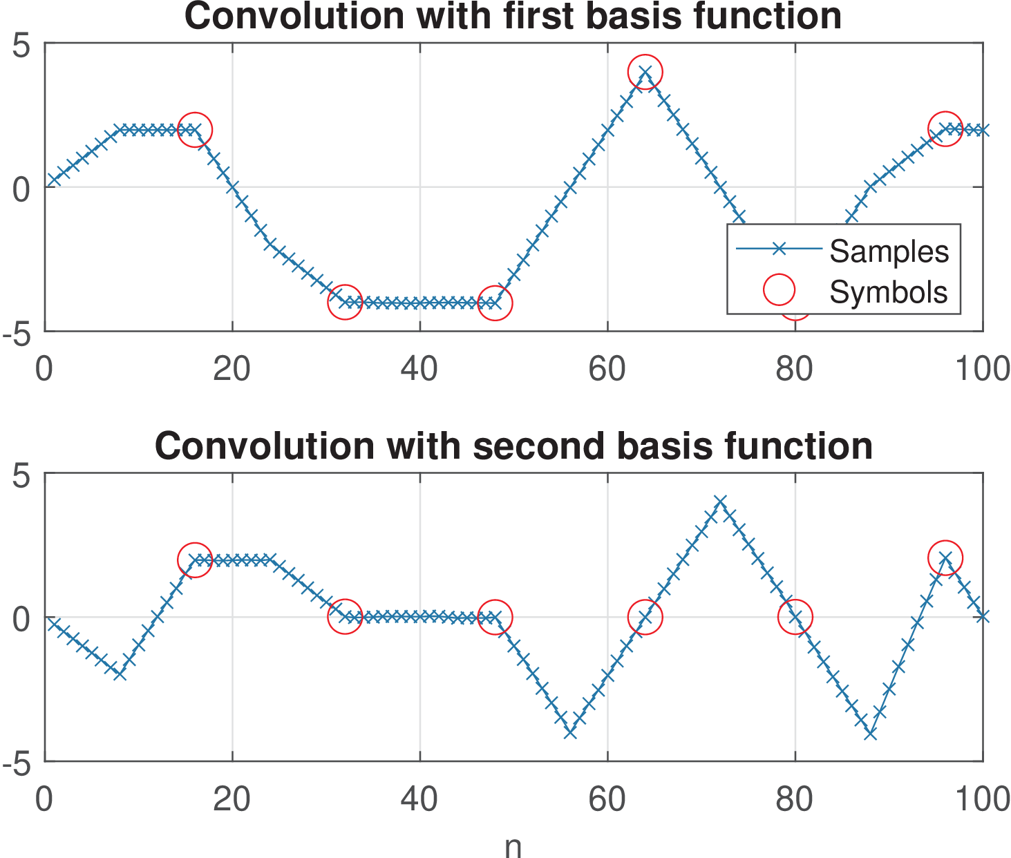
Figure 2.34 shows the convolution output for both basis functions. The symbols (indicated as circles) are obtained with a decimation by D=16. It can be seen from Figure 2.34 (or inspecting m_hat) that the first four decoded symbols are $[2; 2]$ , $[- 4; 0]$ , $[- 4; 0]$ , $[4; 0]$ . To obtain these results, the symbols must be extracted with the proper timing. For example, for the ’conv’ method, the first symbol is at sample $n = 16$ and, after that, at intervals of D=16 samples, the convolution outputs coincide with the desired inner product of the received signal r with the basis functions. $□$

Application 2.9. Cyclostationary analysis in frequency domain. The next paragraphs explore the spectral-correlation density function (SCD), which allows to observe “hidden” periodicities that are not observable via the PSD [Gar91]. The SCD is also discussed in Section A.19.3 and a motivation for using cyclostationary analysis for carrier recovery is described in Listing 4.19.

Listing 2.23 illustrates the SCD estimation using the companion autofam.m function, which implements the FFT Accumulation Method (FAM) [RBLJ91] and is similar to the one implemented in the GNU Radio Spectral Estimation Toolbox [ url9grs].

Listing 2.23: MatlabOctaveCodeSnippets/snip_psd_cyclostationary.m

1numberOfSymbols = 1000;   %number of symbols to be transmitted 
2Fc = 1000; %carrier frequency (Hz) 
3Fs = 8000; %sampling frequency (Hz) 
4df = 80;   %frequency resolution (see [Gardner, 1991]) 
5dalpha = 20; %cyclic frequency resolution 
6L = 12;  %oversampling factor 
7b=4; %number of bits per symbol 
8pulseOption=2; %Choose a pulse option=1 or 2 
9%% Generate PAM signal 
10Rsym = Fs/L; %symbol rate (bauds) 
11M=2^b; %constellation order 
12symbolIndicesTx = floor(M*rand(1,numberOfSymbols)); %random symbols 
13constellation = pammod(0:M-1, M); %PAM constellation 
14symbols = pammod(symbolIndicesTx,M); %obtain PAM symbols from indices 
15%convert symbols into a waveform. 
16switch pulseOption 
17    case 1 
18        p = ones(1,L); %define a simple rectangular shaping pulse 
19    case 2 
20        r = 0.5; % Roll-off factor 
21        delay = 3; %group delay in symbles (at Rsym) 
22        p = ak_rcosine(Rsym,Fs,'fir/normal',r,delay); 
23end 
24p = p / (mean(p.^2)); %make sure pulse has unitary power 
25signal = zeros(1,numberOfSymbols*L); %pre-allocate space 
26signal(1:L:end) = symbols; %organize the symbols 
27signal = filter(p,1,signal); %pulse shaping filtering 
28wc=2*pi*Fc; %carrier frequency in rad/s 
29x = real(signal.*exp(1j*wc*(0:length(signal)-1)*(1/Fs))); 
30%%Cyclostationary analysis 
31[Sx, alphao, fo] = autofam(x,Fs,df,dalpha); %estimate the SCD 
32cyclicProfile = max(Sx,[],1); %estimate the cyclic profile 
33figure(1), plot(alphao,cyclicProfile/max(cyclicProfile));

The SCD is a two-dimensional function that depends on frequency $f$ and “cycle” frequency $α$ . After executing Listing 2.23, the SCD in Figure 2.35 (see, e. g., [Gar91] for further discussion) was obtained with the command

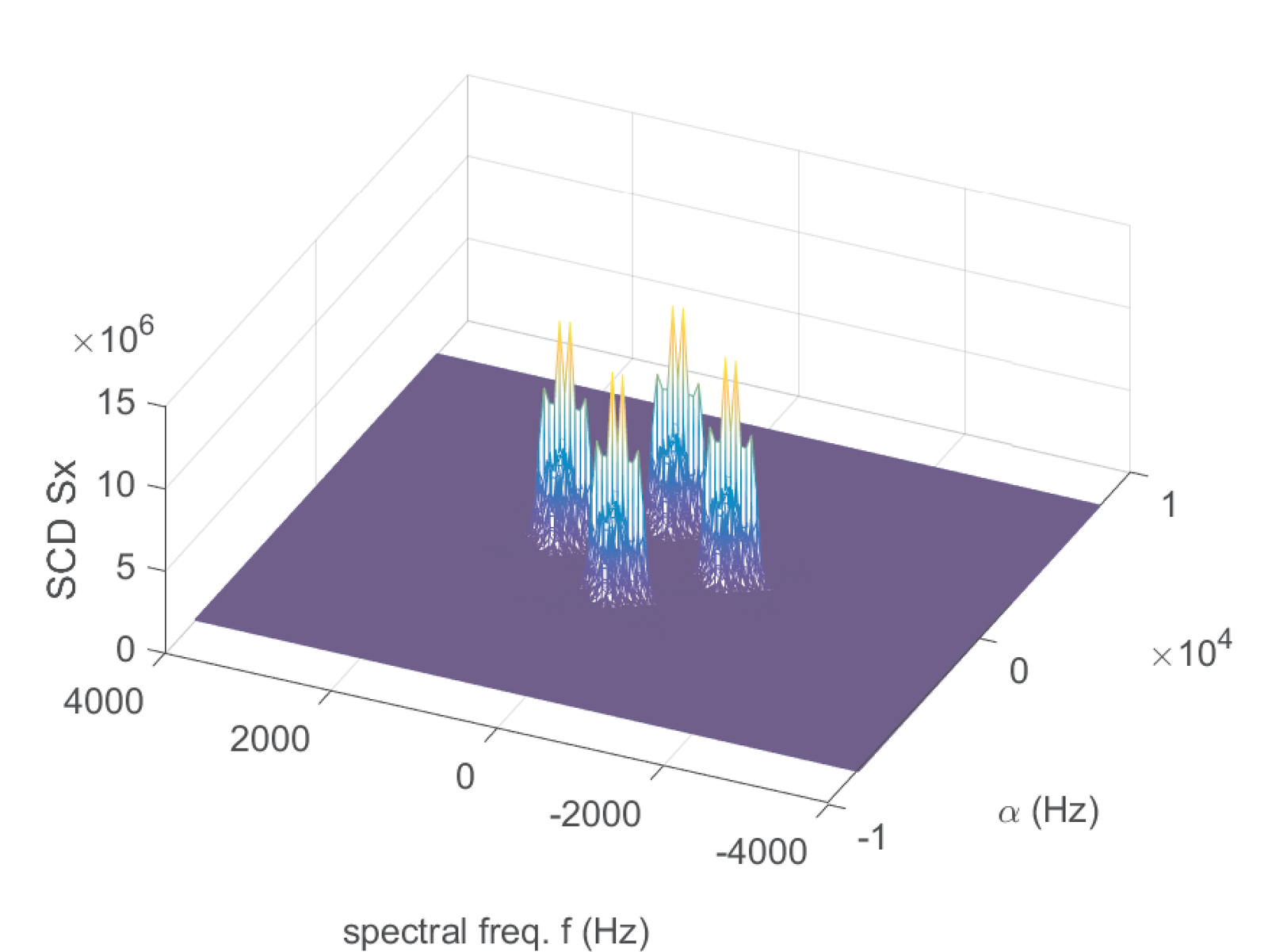
1mesh (alphao,fo, Sx, 'EdgeColor', 'interp');

Figure 2.35: Spectral-correlation density function (SCD) for 16-PAM signal with a carrier frequency of $f_{c} = 1$ kHz.

Given that the carrier frequency is $f_{c} = 1$ kHz, one can observe spectral lines at the cycle frequency $α = 2 f_{c} = 2$ kHz. The maximum value over all frequencies $f$ for each $α$ can be used to define a cyclic or $α$ -profile that can then used to identify the adopted modulation [FGR05].

Figure 2.36: Cyclic profile for the 16-PAM signal in Figure 2.35, which has a carrier frequency

f_{c} = 1

kHz. Note the spectral line at

2 f_{c}

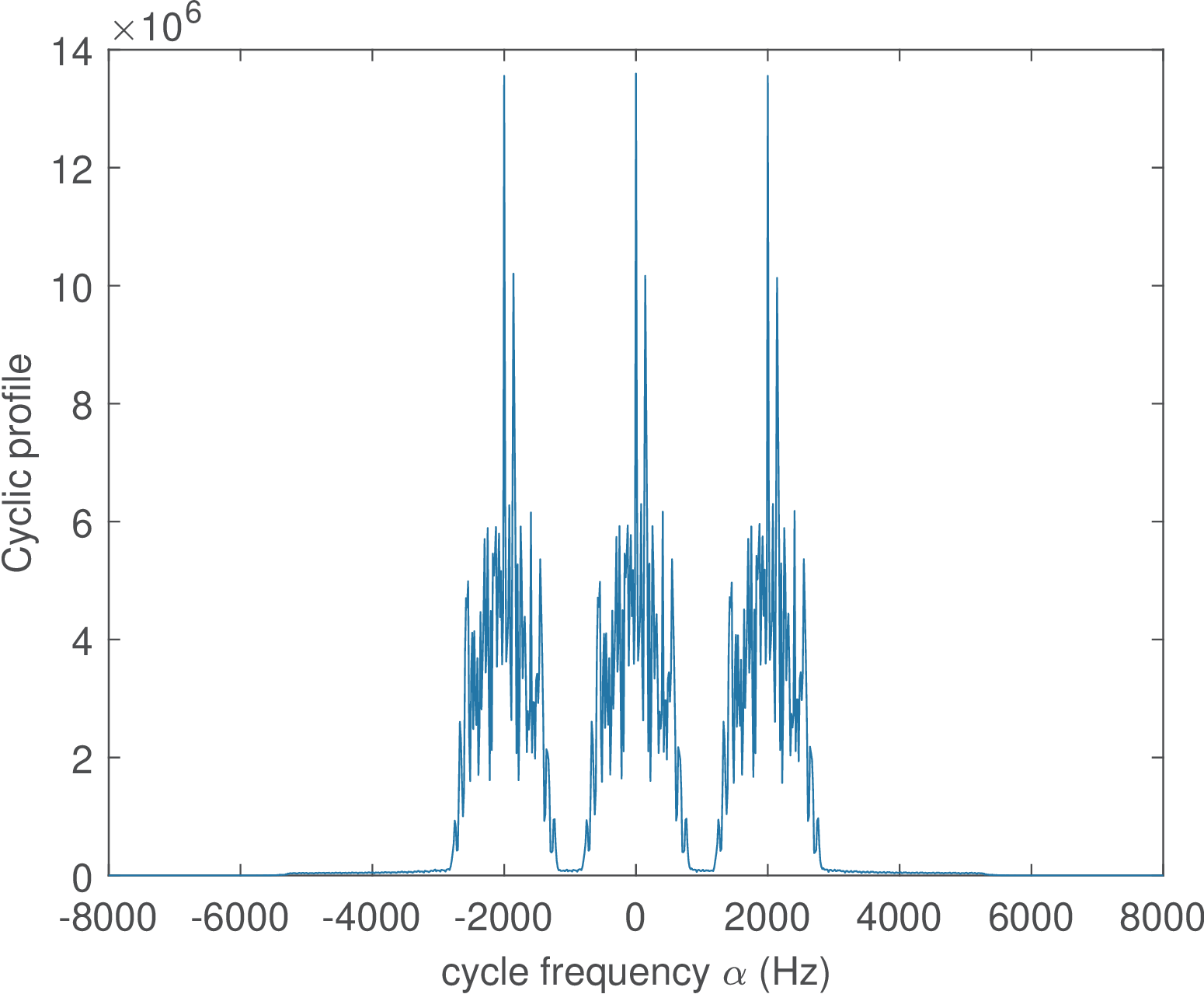
Figure 2.36 shows the result of converting Figure 2.35 to the one-dimensional representation provided by its respective cyclic profile. $□$