M-PAM: A Concrete Example of Digital Modulation

2.7 M-PAM: A Concrete Example of Digital Modulation

Pulse amplitude modulation (PAM) is the generic term adopted for a set of techniques that allow to transport information via the amplitude of a waveform. For example, in analog PAM systems, an analog waveform $m (t)$ carrying information in its amplitude is multiplied by a periodic pulse train. In this text, the emphasis is on digital $M$ -ary PAM systems, which for simplicity are called PAM systems hereafter.

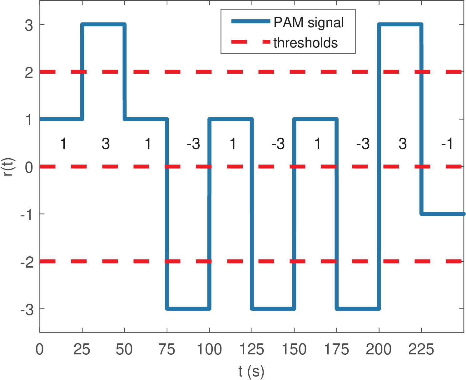
Figure 2.4: Example of received M-PAM signal with symbol duration $T_{sym} = 25$ s and symbols $M = {- 3, - 1, 1, 3}$ . The decision thresholds are ${- 2, 0, 2}$ .

Figure 2.4 shows an example of an $M$ -PAM signal $r (t)$ with $M = 4$ symbols composing the set $M = {- 3, - 1, 1, 3}$ . For each symbol interval $T_{sym}$ , which in this case is $T_{sym} = 25$ s, the amplitude of the PAM waveform is obtained from $M$ and is held constant for the corresponding $T_{sym}$ . The PAM signal in Figure 2.4 is assumed to be arriving at the receiver, which corresponds to the ideal situation of receiving a noiseless signal without any distortion. The set of symbols $M$ , known by both transmitter and receiver, allows the receiver to use the sensible strategy of guessing which symbol of $M$ was transmitted by comparing the amplitude of the received signal to the decision thresholds ${- 2, 0, 2}$ . For example, if the amplitude lies between $- 2$ and 0, the receiver assumes the transmitted symbol was $- 1$ . These decisions must be done periodically at a rate $R_{sym} = 1 ∕ T_{sym}$ , which is called the symbol rate.

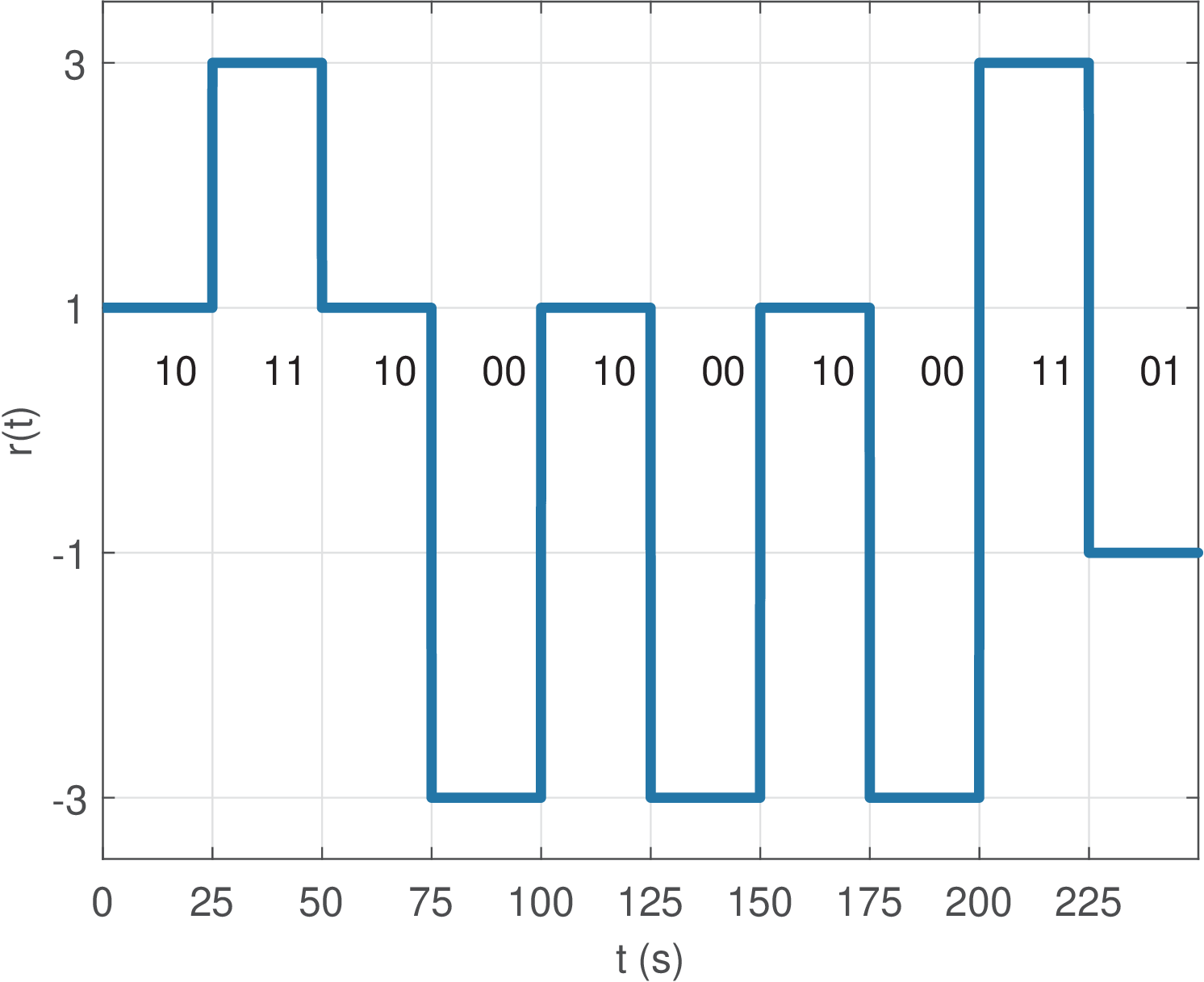
The advantage of departing from binary systems and using $M > 2$ symbols is the capability of transporting $b = {log}_{2} M$ bits per symbol. In the signal of Figure 2.4, $b = {log}_{2} 4 = 2$ bits can be mapped such that the amplitudes ${- 3, - 1, 1, 3}$ can be related to the bits ${00, 01, 10, 11}$ , respectively. A constellation is fully specified by the set $M$ and the assignment of bits (or codewords) to the symbols in $M$ . Figure 2.5 is a version of Figure 2.4 that shows the binary codes used for each amplitude. It can be observed that the demodulated bitstream is 10 11 10 00 10 00 10 00 11 01 and, given the received and transmitted signals are the same in this ideal situation, the bit error rate (BER) is zero. In this case, the bit rate $R$ in number of bits per second (bps) can be found by noting that $R_{sym}$ symbols are received per second and each symbol carries $b$ bits, which leads to $R = b R_{sym} = 2 (1 ∕ 25) = 0.08$ bps.

Figure 2.5: Version of Figure 2.4 that shows the pair of bits that the amplitude of each symbol represents.

Figure 2.6: Version of Figure 2.4 with a dispersive channel that introduces distortion and delays the transmitted signal.

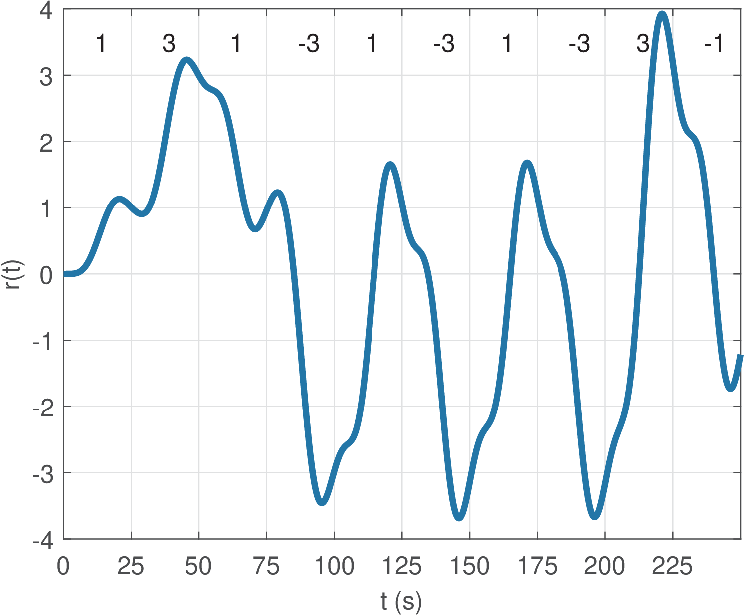
Note from Figure 2.5 that due to the assumed ideal situation, it is easy to observe where each symbol starts and ends. However, the practical transmission systems have some degree of channel dispersion, which loosely speaking means that the channel will delay and distort the signal such that a symbol can interfere with subsequent symbols. Note that channel dispersion can be observed when the channel impulse response differs from an impulse and can be interpreted in frequency-domain as a non-flat frequency response. Hence, a frequency-selective channel corresponds to a dispersive channel. Figure 2.6 shows an example where the signal of Figure 2.4 was transmitted over a system $H (z)$ (a Chebyshev filter obtained with cheby1). This is a situation where there is no noise, only channel dispersion, but it is clearly harder to demodulate the signal. The first point is that there is a delay imposed by the channel. For example, the first symbol is not limited to the interval from 0 to 25 s, as in Figure 2.5.

The delay imposed by a channel is discussed in Applications E.6 and E.10. For the channel used to generate Figure 2.6, the group delay (estimated with grpdelay) is approximately 12 s around DC, increases up to 25 s at 0.06 Hz and is approximately zero for frequencies higher than 0.3 Hz. The overall effect of these influences in the frequency components of the input signal generates the situation of Figure 2.6, where the amplitude of the intended symbol is better visualized almost at the end of the corresponding original time interval. For example, a maximum amplitude of 1.13 corresponding to the first symbol is observed around 20.8 s while the second received symbol has a peak of amplitude 3.23 at 45.4 s.

A pertinent question is how to estimate the channel delay in practice, especially in situations such as wireless communications where this delay varies over time. One approach is based on cross-correlation. As done in Application C.13, using the function xcorr for the transmitted and received signals of Figure 2.6 indicates that the correlation has a peak at a lag corresponding to 12.6 s. This kind of information can be used by the receiver to determine an instant of reference for demodulating the symbols.

The next paragraphs correspond to a hands-on discussion of PAM-based systems, where the reader is invited to execute short codes in Matlab/Octave to get familiar with important concepts.

2.7.1 Generation of symbols from a PAM constellation

Any set of $M$ distinct real numbers can be used to constitute a PAM constellation. An example could be $M = {- 1.4, 3.2, 16.0}$ , with $M = 3$ . But in practice, a PAM constellation obeys the following guidelines:

the constellation order $M = 2^{b}$ is a power of 2, where $b$ is the number of bits per symbol;
the distance $d$ between neighboring symbols is the same;
the symbols average is zero, i. e., $\frac{1}{M} \sum_{m = 1}^{M} m_{i} = 0$ ;
when relating the symbols to their binary representation, Gray coding is used to aim at a smaller number of bit errors (BER) when a symbol error occurs.

Using $d = 2$ is convenient and adopted in many situations. In case $d = 2$ , the PAM symbols can be generated in Matlab/Octave with the command -(M-1):2:M-1 and later normalized to have a specified distance $d$ or constellation energy

{\bar{E}}_{c} ≜ 𝔼 [| m_{i} |^{2}]

(2.9)

Considering that all symbols are equiprobable leads to Eq. (C.69).

While PAM symbols are real numbers, this definition of ${\bar{E}}_{c}$ uses the modulus $|⋅|$ to take into account that other modulations use complex symbols.

For example, Listing 2.2 illustrates how to obtain two sets of constellation symbols from symbols spaced by $d = 2$ : the first set cx with $d = 8$ and another set cy with ${\bar{E}}_{c} = 20$ J.

Listing 2.2: MatlabOctaveCodeSnippets/snip_digi_comm_PAM_constellation.m

1M=4 %modulation order 
2canonicalPAMSymbols = -(M-1):2:M-1 %original, Delta = 2 
3cx = canonicalPAMSymbols/2; %intermediate result, Delta=1 
4cx = 8 * cx %convert to the specified Delta=8 
5originalEnergy = mean(abs(canonicalPAMSymbols).^2); 
6cy = canonicalPAMSymbols / sqrt(originalEnergy); %Ec = 1 
7cy = sqrt(20) * cy %convert to the specified Ec=20 J

Note that after transmission over a channel, the received signal can be significantly attenuated and, before the detection stage, it may be necessary to use an AGC or normalize the received symbols to have the energy (or power) assumed by the detection stage.

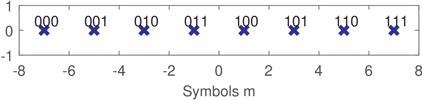
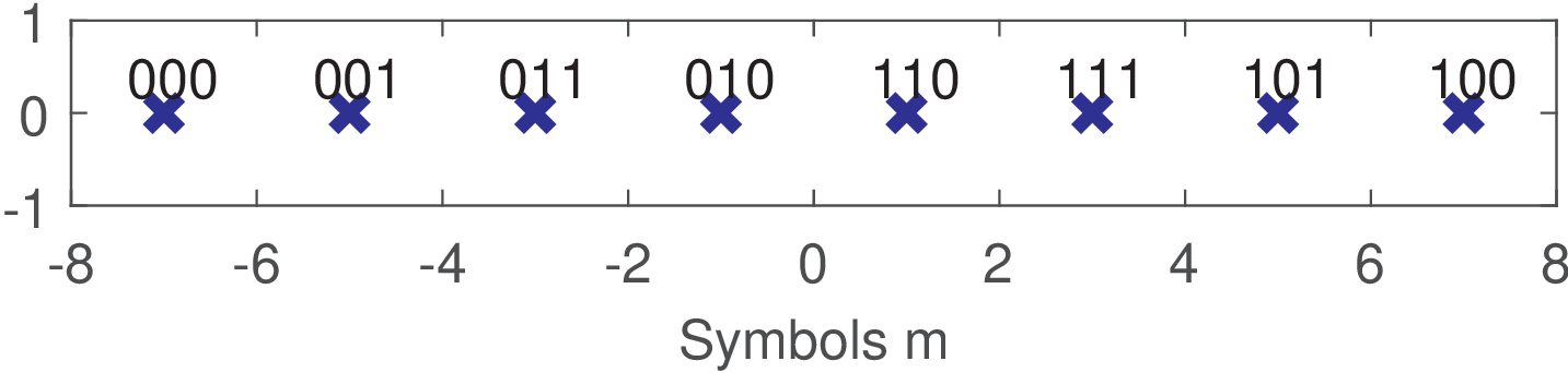
Up to now, the discussion was restricted to the set of symbols of a constellation. To completely specify the constellation, its symbols must be associated to bits. Figure 2.7 shows an example for 8-PAM with $d = 2$ . The assignment of bits to each symbol uses the natural order. The first (left-most) symbol $- 7$ corresponds to 0 in decimal, $- 5$ corresponds to 1, etc. Hence, $- 7$ is 000, $- 5$ is 001 and so on. One can observe that identifying individual symbols using the decimal or binary representation depends only on convenience. The Matlab/Octave functions dec2bin and bin2dec help converting between these two representations.

In the GNU Radio (GR) platform, as discussed in Application 2.3, the bits are typically packed into integers that are called chunks.

Note that if the symbol $- 1$ (representing the bits 011) gets confused at the receiver by its neighbor symbol 1 (bits 100), there are three bit errors. When one considers the presence of noise, it is interesting to use Gray coding and aim at achieving the performance predicted by Eq. (2.4).

Table 2.1 contrasts the natural and Gray representations. In Matlab/Octave, the Gray code can be conveniently generated with the command M=8; alphabet = pammod(0:M-1,M,0,’gray’) that results in [-7,-5,-1,-3,7,5,1,3]. For this constellation, a chunk in Gnu Radio of integer value 2 (or 010 in binary) represents the symbol $- 1$ . Figure 2.8 illustrates a Gray-coded constellation.

Table 2.1: Example of Gray coding for 8-PAM.

Symbol m	-7	-5	-3	-1	1	3	5	7
Natural decimal representation	0	1	2	3	4	5	6	7
Natural binary representation	000	001	010	011	100	101	110	111
Gray decimal representation	0	1	3	2	6	7	5	4
Gray binary representation	000	001	011	010	110	111	101	100

Figure 2.7: Example of 8-PAM constellation using natural order.

Figure 2.8: Gray-coded 8-PAM constellation.

The random generation of a large number of PAM symbols in Matlab/Octave is relatively simple and can be done with a code such as Listing 2.3.

Listing 2.3: MatlabOctaveCodeSnippets/snip_digi_comm_random_symbols.m

1M=8; %modulation order 
2N=10000; %number of symbols to be generated 
3indices=floor(M*rand(1,N))+1; %random indices from [1, M] 
4alphabet=[-(M-1):2:(M-1)]; %symbols ...,-3,-1,1,3,5,7,... 
5m=alphabet(indices); %obtain N random symbols

Listing 2.3 uses the function rand to generate uniformly distributed random indices and the syntax m=alphabet(indices) to obtain their corresponding symbols.

2.7.2 Average energy of PAM constellations

Assuming that practical PAM constellations have uniformly-spaced symbols with distance $d$ between neighbors, the average constellation energy ${\bar{E}}_{c}$ depends only on $d$ and $M$ and Eq. (2.9) can be specialized to this case.

To calculate ${\bar{E}}_{c}$ for the uniformly-spaced PAM constellation $\pm \frac{d}{2}, \pm \frac{3 d}{2}, \pm \frac{5 d}{2}, \dots, \pm \frac{(M - 1) d}{2}$ where $M = 2^{b}$ is an even number, one should note that there are $M ∕ 2$ pairs of symbols with energy $k^{2} d^{2} ∕ 4$ , where $k$ is an odd number: $k = 1, 3, \dots, M - 1$ . Therefore,

\begin{align} {\bar{E}}_{c} & = (\frac{1}{M}) 2 \sum_{i = 1}^{M ∕ 2} {(2 i - 1)}^{2} \frac{d^{2}}{4} \\ = \frac{d^{2}}{2 M} \sum_{i = 1}^{M ∕ 2} (4 i^{2} - 4 i + 1) . \end{align}

About the three parcels in the above summation, the second one (corresponding to $- 4 i$ ) can be calculated from the arithmetic series $\sum_{i = 1}^{M ∕ 2} i = \frac{M ∕ 2 (M ∕ 2 + 1)}{2}$ . The first one (corresponding to $4 i^{2}$ ) can use Eq. (A.17), which indicates that the sum of squares is $\sum_{i = 1}^{M ∕ 2} i^{2} = \frac{M ∕ 2 (M ∕ 2 + 1) (M + 1)}{6}$ . With these two results and after some algebra one gets

{\bar{E}}_{c} = \frac{d^{2} (M^{2} - 1)}{12} .

(2.10)

2.7.3 PAM detection

When using the traditional PAM constellations, in which every symbol has the same distance $d$ from its neighbors, the detection is relatively simple, as shown in Listing 2.4 for $d = 2$ .

Listing 2.4: MatlabOctaveFunctions/ak_pamdemod.m

1function [symbolIndex, x_hat]=ak_pamdemod(x,M) 
2% function [symbolIndex, x_hat]=ak_pamdemod(x,M) 
3%Inputs: x has the PAM values and M the number of symbols 
4%Outputs: symbolIndex has the indices from 0 to M-1 
5%         x_hat contains the nearest symbol(s) 
6delta = 2; %assume symbols are separated by 2 
7symbolIndex = (x+M-1) / delta; %quantizer levels 
8symbolIndex=round(symbolIndex); %nearest integer 
9symbolIndex(symbolIndex > M-1) = M-1; %impose maximum 
10symbolIndex(symbolIndex < 0) = 0; %impose minimum 
11if nargout > 1 %calculate only if necessary 
12    x_hat = (symbolIndex * delta)-(M-1);%quantized output 
13end

In this case, the PAM detection is equivalent to a uniform quantization. The only distinction between PAM detection and Listing C.18 is that the quantization stairs is shifted because “zero” is not a PAM symbol.⁹

If the constellation does not have the same distance among neighboring symbols, the computational cost of detection increases. Listing 2.5 illustrates how to choose the decoded symbol for a generic constellation, by picking the symbol with the smallest Euclidean distance to the input value.

Listing 2.5: MatlabOctaveFunctions/ak_genericDemod.m

1function [symbolIndex, x_hat]=ak_genericDemod(x,constel) 
2% function [symbolIndex, x_hat]=ak_genericDemod(x,constel) 
3%Finds the nearest-neighbor symbol for any constellation. 
4%Inputs:  x the symbols (PAM, QAM or 3d-vectors, etc) to be 
5%         "demodulated", one per column (PAM and QAM can be vectors 
6%         with real and complex numbers, respectively). 
7%         constel - constellation with a symbol per column 
8%Outputs: symbolIndex has the indices from 0 to M-1, where 
9%         x_hat has the nearest symbol(s) and same dimension as x 
10%Usage: 
11%x=[2,2+4j,-1,-1,-j], c=[1,j,-1,-j], [s,x_hat]=ak_genericDemod(x,c) 
12%x=rand(3,5); c=[1 0;0 1;1 1]; [s,x_hat]=ak_genericDemod(x,c) 
13if isvector(x) 
14    S=length(x); %number of symbols (PAM or QAM) in x 
15    if ~isvector(constel) 
16        error('Constellation must be a vector if input is a vector'); 
17    end 
18    x=transpose(x(:)); %make sure x is a row vector 
19    constel=transpose(constel(:)); %make sure constel is a row vector 
20    M=length(constel); %number M of symbols in constellation 
21    D=1; %assume dimension is 1 
22else 
23    [D,S]=size(x); %S symbols of dimension D are organized in columns 
24    [D2,M]=size(constel); %get number M of symbols in constellation 
25    if D ~= D2 
26        error('Dimension (number of rows) must be same for inputs'); 
27    end 
28end 
29symbolIndex=zeros(1,S); %pre-allocate space for S indices 
30x_hat=zeros(D,S); %pre-allocate space for S symbols of dimension D 
31for i=1:S %loop over all S input vectors in x 
32    bestSymbolIndex = 1; %temporarily assume first symbol as closest 
33    minDistance=norm(x(:,i)-constel(:,bestSymbolIndex),2);%initialize 
34    for j=2:M %search all other symbols in constellation 
35        distance = norm(x(:,i)-constel(:,j),2); %Euclidean distance 
36        if distance < minDistance %update best symbol if true 
37            minDistance = distance; %update minimum distance 
38            bestSymbolIndex = j; %store best symbol index 
39        end 
40    end 
41    symbolIndex(i)=bestSymbolIndex-1; %store best symbol index 
42    x_hat(:,i)=constel(:,bestSymbolIndex); %and corresponding symbol 
43end

Note that, for example, the two functions invoked in the following code give the same result, but ak_pamdemod is faster because it can take into account the symbols are uniformly spaced.

1x=[1.1, -4, 7]; %some arbitrary vector to test the two functions 
2[a,b]=ak_pamdemod(x,4) %function assumes symbols are uniformly spaced 
3[a,b]=ak_genericDemod(x,[-3 -1 1 3])%supports arbitrary constellation

2.7.4 Symbol-based PAM simulation

As discussed, samples and symbols are distinct elements of a digital communication system. Samples compose waveforms while symbols carry information and are restricted to be elements of a given constellation. Hence, one must distinguish two distinct rates: the sampling frequency $F_{s}$ and the symbol rate $R_{sym}$ or, equivalently, the sampling $T_{s} = 1 ∕ F_{s}$ and symbol $T_{sym} = 1 ∕ R_{sym}$ intervals, respectively.

Based on symbols and samples, two important simulation strategies will be discussed: symbol-based and sample-based (or oversampled) simulations. For a symbol-based simulation, the vector representing the transmit signal is composed not by samples, but by the symbols themselves, and the time interval between consecutive elements is not $T_{s}$ , but $T_{sym}$ . The symbol-based often demands less computation than the sample-based simulations, as discussed in the sequel.

The symbol-based simulation model is based on sending the symbols directly to a channel that accepts symbols at its input and outputs symbols. In this case, the sampling interval $T_{s}$ is not defined or, if convenient, it can be thought as equal to the symbol rate, i. e., $T_{s} = T_{sym}$ .

As a “sanity check”, Listing 2.6 provides a transmission example without noise nor distortion. It illustrates a situation where the received symbols are made equal to the transmitted symbols. The variable numberOfErrors is zero, as expected in this case.

Listing 2.6: MatlabOctaveCodeSnippets/snip_digi_comm_tx_rx_comparison.m

1M=16; %modulation order 
2numberOfSymbols = 40000; % number of symbols 
3alphabet = [-(M-1):2:M-1]; %M-PAM constellation 
4symbolIndicesTx = floor(M*rand (1, numberOfSymbols )); 
5s = alphabet(symbolIndicesTx +1); %transmit signal 
6r = s; %no channel: received = transmit signal 
7symbolIndicesRx = ak_pamdemod(r, M);% demodulate 
8numberOfErrors = sum(symbolIndicesTx ~= symbolIndicesRx)

The AWGN channel can easily operate at the symbol-level. As exemplified in Listing 2.7, random noise n can be directly added to the transmitted symbols s such that the received symbols are r=s+n. Note that, in this case, each symbol can be considered a waveform sample, but it is important to keep distinguishing the concepts of symbol and sample.

Listing 2.7: MatlabOctaveCodeSnippets/snip_digi_comm_Symbol_Error_Rate.m

1randn('state',0); rand('state',0);%reset random generators 
2M=16; %modulation order 
3numSymbols = 40000; % number of symbols 
4alphabet = [-(M-1):2:M-1]; %M-PAM constellation 
5symbolIndicesTx = floor(M*rand(1, numSymbols)); %random indices 0:M-1 
6s = alphabet(symbolIndicesTx + 1); %transmit symbols (indices 1 to M) 
7Pn = 2 %noise power (assumed to be in Watts) 
8n = sqrt(Pn)*randn(size(s)); %white Gaussian noise 
9r = s+n; %channel with additive white Gaussian noise 
10symbolIndicesRx = ak_pamdemod (r, M);% demodulate 
11SER = sum(symbolIndicesTx~=symbolIndicesRx)/numSymbols %symbol errors 
12Ps = mean(alphabet.^2) %transmit signal power (Watts) 
13Pr = mean(r.^2) %received signal power (Watts) 
14SNR = Ps/Pn %SNR in linear scale 
15N0_s = 10*log10(Ps/pi) %unilateral Tx PSD level in log scale 
16N0_r = 10*log10(Pr/pi) %unilateral Rx PSD level in log scale 
17N0_n = 10*log10(Pn/pi)%unilateral PSD noise level in log scale

Executing Listing 2.7 leads to SER=0.45, which is rather high. Observing the received constellation with plot(real(r),imag(r),’x’) would illustrate the noise is too intense.

Note that for improved efficiency the signal power $P$ was obtained with mean(alphabet. $\hat{}$ 2), which is the constellation energy ${\bar{E}}_{c}$ as dictated by Eq. (C.69).¹⁰ The power $P$ could also be obtained with mean(s. $\hat{}$ 2) but given that $P \approx {\bar{E}}_{c}$ in this case, the former method is faster. Note that, asymptotically, when numSymbols goes to infinity, $P = {\bar{E}}_{c}$ in symbol-based PAM simulations. The more general case of finding the power of sample-based PAM signals is discussed in Section 2.7.8.

2.7.5 Flat PSD of symbol-based PAM signals

They are faster than sample-based simulations, but one important limitation of symbol-based simulations is that there is no control of the transmit signal spectrum. The implicit assumption that $T_{s} = T_{sym}$ and of statistical independence of the symbols leads to a flat (white) PSD because the signal autocorrelation $R [l]$ is, theoretically, non-zero only at lag $l = 0$ . Hence, a sequence of PAM symbols has the same PSD as white noise and the concepts in Section F.7.3 apply here.¹¹

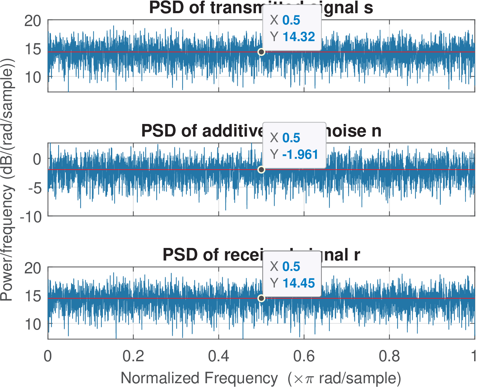
Figure 2.9: Power spectral densities (in dB/rad) for the transmit, noise and received signals.

For Listing 2.7, the transmit, noise and received signals had power $P_{s} = 85$ , $P_{ν} = 2$ and $P_{r} = 87.5$ W, respectively. Figure 2.9 shows the one-sided PSDs obtained by commands pwelch. Because the noise and transmitted signals are uncorrelated, one can apply Eq. (C.76) and observe that $P_{r} \approx P_{s} + P_{ν}$ . The transmit PSD has an average value (recall that, by default, pwelch returns unilateral PSDs) of $N_{0} = 10 {log}_{10} (85 ∕ π) \approx 14.3$ dB/normalized frequency. Similarly, the values of $N_{0}$ for the noise and received signals are 4.4 and 14.7 dB/normalized frequency, respectively, which are indicated by horizontal lines in Figure 2.9. Note that $P_{r} = P_{s} + P_{ν}$ is applied with powers in linear scale (Watts), not in dB, and a similar reasoning applies when adding PSDs.

It can be proved that in some cases the performance of a PAM system can be evaluated by an equivalent symbol-based representation.¹² However, to assess aspects such as channel equalization, it would be a limiting factor to simulate a communication system only with flat PSDs. Oversampling is used to circumvent this restriction. The next section discusses sample-based simulations, which allow using signals with non-flat PSDs. PAM is assumed for simplicity.

2.7.6 Sample-based (oversampled) PAM simulation

This section deals with the generation and demodulation of PAM signals with a spectrum imposed by a shaping pulse $p [n]$ (or $p (t)$ in continuous-time). Oversampling is a required condition for having control of the transmit signal spectrum.

In the oversampled case, $T_{sym} > T_{s}$ and the ratio

L = \frac{T_{sym}}{T_{s}}

(2.11)

is called the oversampling factor. Its choice depends on several aspects, such as the bandwidth of the signals used to represent information. In many communication device firmwares, such as the modem of a handset, for example, the oversampling is an integer in the range $L \in [2, 16]$ . Higher values of $L$ may be used during simulation-based studies though.

Assuming discrete-time, $L > 1$ samples are used to describe the waveform segment that represents a single symbol. While a symbol-based simulation has $L = 1$ and a transmit signal that has a flat spectrum, the extra degree of freedom provided by $L > 1$ allows to shape this spectrum, as desired.

The majority of the PAM systems generates the $n$ -th waveform segment $s_{n} (t)$ or $s_{i} [n]$ via the simple expressions

s_{i} (t) = m_{i} p (t) or s_{i} [n] = m_{i} p [n],

(2.12)

respectively, where $m_{i}$ is the $i$ -th symbol (e. g., two values, representing bits 0 and 1 in case of a binary system) and $p (t)$ or $p [n]$ is a formatting pulse.

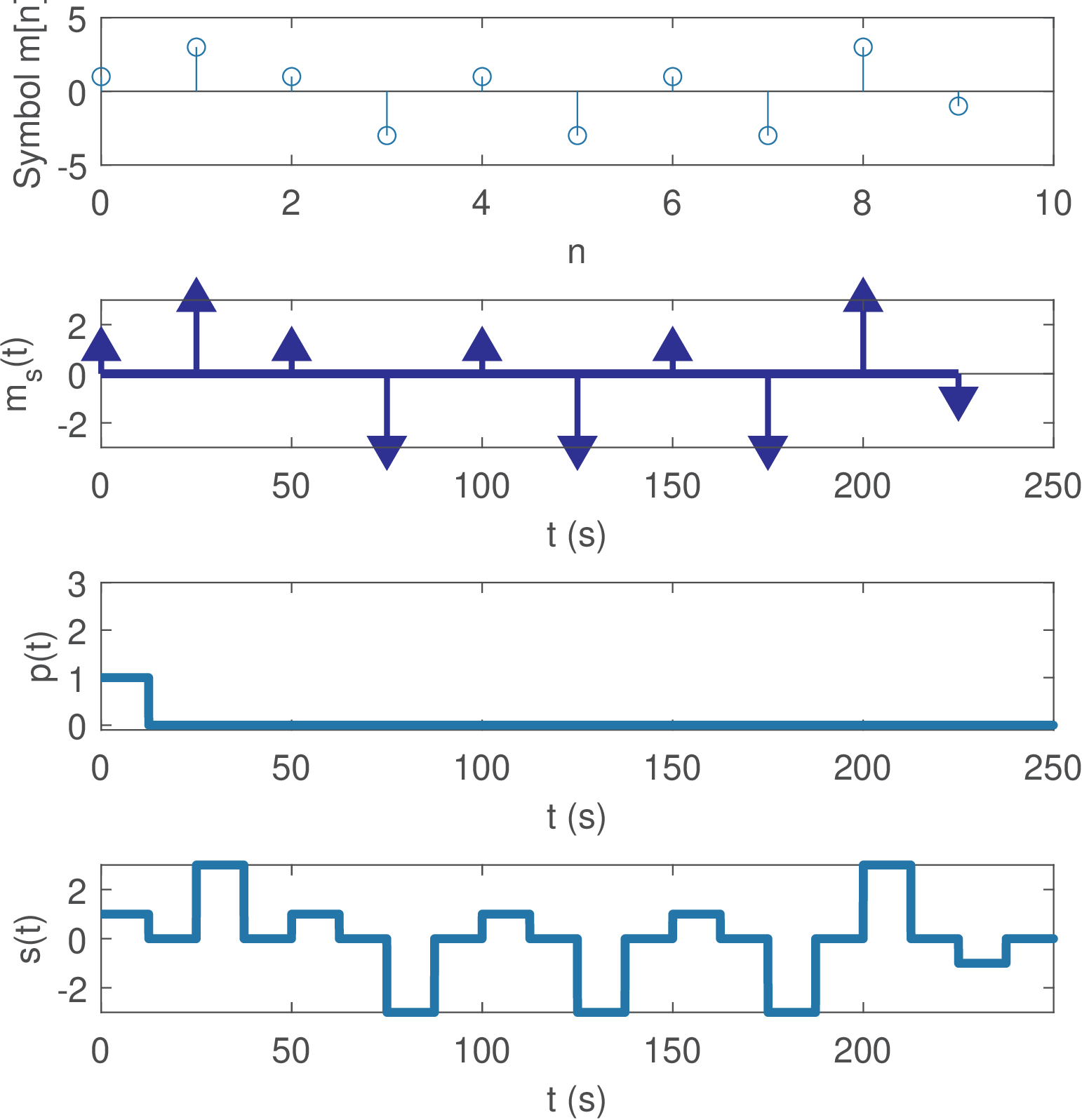
Figure 2.10: Continuous-time PAM $s (t)$ generated with $T_{sym} = 25$ s. The pulse $p (t)$ has amplitude one and support [0, 12.5[ s.

Figure 2.10 illustrates an example of PAM with $T_{sym} = 25$ s ( $R_{sym} = 0.04$ bauds) and a pulse $p (t)$ with support from 0 to 12.5 s and amplitude 1. Observe that a new symbol is transmitted at every $T_{sym}$ , but the transmitted waveform $s (t)$ exists for all $t$ and depends on both the symbols and shaping pulse $p (t)$ . The pulse in Figure 2.10 has support $T_{sym} ∕ 2$ such that $s (t)$ is called a RZ (return-to-zero) signal. If the spectrum of $s (t)$ needs to obey constraints, they can imposed by controlling $p (t)$ and also the statistical properties of the symbols $m [n]$ . This leads to several distinct families of transmitted signals, which are called line codes, as will be seen in Section 2.10.

2.7.7 Interpreting the shaping pulse as the impulse response of a LIT

For continuous-time processing and assuming an infinite sequence of symbols $m [i]$ , the PAM signal is given by:

s (t) = \sum_{i = - \infty}^{\infty} m [i] p (t - i T_{sym}) .

(2.13)

Similarly, for discrete-time processing:

s [n] = \sum_{i = - \infty}^{\infty} m [i] p [n - iL],

(2.14)

where $L$ is the oversampling factor defined in Eq. (2.11).

The generation of an oversampled PAM signal is a little more involved than a symbol-based PAM. It can be interpreted as an interpolation process and, consequently, it may be tempting to use a function such as interp, which implements upsampling and filtering. However, it is recommended to explicitly deal with the shaping pulse $p [n]$ (that typically represents $p (t)$ ) and do not use interp or similar functions.

In continuous-time, the PAM generation uses a D/C conversion to obtain a sampled signal $m_{s} (t)$ with sampling interval $T_{sym}$ from a discrete-time sequence of symbols $m [n]$ , as indicated in

m [n] \to D/C \to m_{s} (t) \to p(t) \to s (t) .

(2.15)

The signal $p (t)$ can be interpreted as the impulse response of a LTI system, and this interpretation will be often used hereafter. The convolution of $m_{s} (t)$ with $p (t)$ provides the PAM signal $s (t)$ . The observation of the signals described in Figure 2.10, which depicts $s (t) = m_{s} (t) * p (t)$ , helps to interpret the process.

A similar approach can be used to generate a discrete-time PAM signal $s [n]$ . In this case, the D/C conversion is substituted by an upsampling operation that inserts zeros between samples of $m [n]$ (do not confuse upsampling with frequency upconversion). Hence, one can obtain the signal $s [n]$ by convolving an upsampled symbols sequence $m_{u} [n]$ with $p [n]$ , as illustrated in:

m [n'] \to ↑ L \to m_{u} [n] \to p[n] \to s [n] .

(2.16)

The notation $m [n']$ indicates that the first signal has an associated sampling interval $T_{sym}$ that is distinct from the interval $T_{s}$ adopted for the other two signals.

The generation of a discrete-time oversampled PAM signal is illustrated in Listing 2.8. Note that both $p [n]$ and $s [n]$ must be associated to the same sampling frequency $F_{s}$ . In other words, when converted to continuous-time, the interval between the original samples of discrete-time signals is the sampling period $T_{s} = 1 ∕ F_{s}$ .

Listing 2.8: ./Code/MatlabOctaveCodeSnippets/snip_digi_comm_pam_generation.m

1M=8; %modulation order (cardinality of the set of symbols) 
2N=10000; %number of symbols to be generated 
3L=3; %oversampling factor 
4indices=floor(M*rand(1,N))+1; %random indices from [1, M] 
5alphabet=[-(M-1):2:M-1]; %symbols ...,-3,-1,1,3,5,7,... 
6m=alphabet(indices); %obtain N random symbols 
7m_upsampled=zeros(1,N*L); %pre-allocate space with zeros 
8m_upsampled(1:L:end)=m; %symbols with L-1 zeros in-between 
9p=ones(1,L); %shaping pulse with square waveform 
10s=conv(m_upsampled,p); %convolve symbols with pulse

The samples of the sequence m in Listing 2.8 are separated by an interval equivalent to $T_{sym}$ . The upsampling operation creates a new sequence m_upsampled in which the samples are separated by an interval of $T_{s}$ . The command s=conv(m_upsampled,p) obtains the desired PAM signal. Note that, as in the continuous-time case, $p [n]$ can be interpreted as the impulse response of a LTI system.

Recall that the convolution of sequences of lengths $N_{1}$ and $N_{2}$ generates a sequence of $N_{1} + N_{2} - 1$ samples. When using s=conv(m_upsampled,p) in Listing 2.8, the vector s has more samples than m_upsampled. If their lengths should be the same (see Section E.15.3), the convolution tail can be eliminated manually (after conv) or by using filter (instead of conv):

1s=filter(p,1,m_upsampled); %convolve and discard tail

In the previous command, the filter command used the fact that the impulse response p of a FIR filter coincides with its coefficients, such that p and 1 are, respectively, the numerator and denominator of the system function $H (z)$ of this filter.

Figure 2.11 shows an example obtained by modifying Listing 2.8. In this case, the oversampling factor $L = 5$ was made longer than the support of $p [n]$ (3 samples), such that $s [n]$ has two zero-valued samples per symbol.

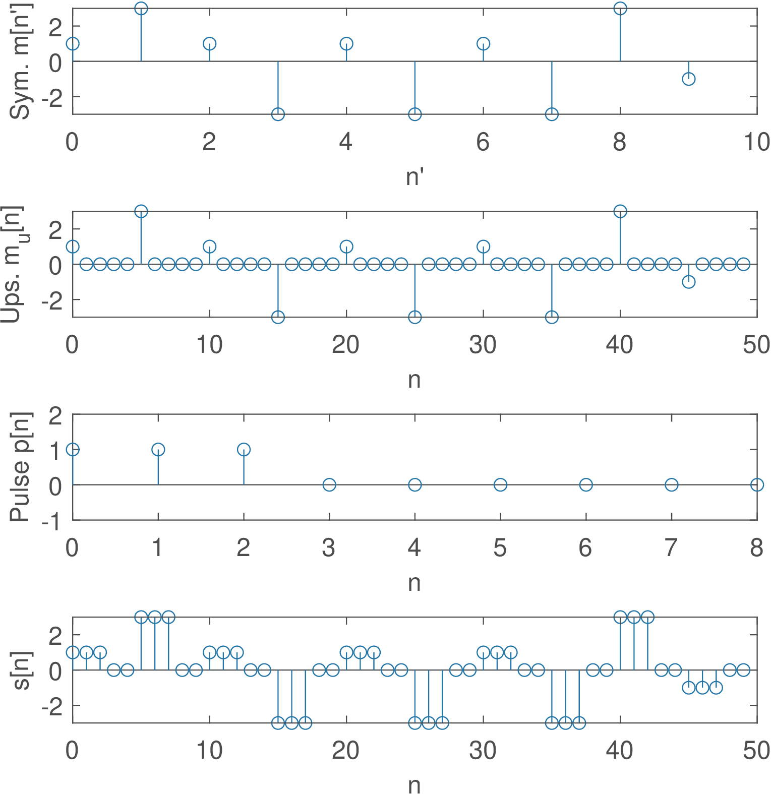
Figure 2.11: Stages of generating a discrete-time PAM signal: 1) random symbols, 2) upsampling, 3) pulse p=[1 1 1], 4) convolution with pulse. The parameters were M=4 possible symbols, N=10 generated symbols, and oversampling L=5.

It should be noticed that Figure 2.11 and Figure 2.10 correspond to distinct representations of signals (discrete and continuous-time, respectively). However, the actual representation when simulating in Matlab/Octave is the discrete-time version of Figure 2.11 given that the simulations represent signals as arrays. For example, Figure 2.10 was obtained in Matlab/Octave using a relatively high oversampling factor $L = 500$ for getting plots that better represent continuous-time signals (with sharp transitions). Continuous-time signals are more naturally represented by tools such as Simulink.

2.7.8 Advanced: Power of PAM signals

Eq. (E.102) can be used to obtain the power of a PAM signal, even if the duration of $p (t)$ (or $p [n]$ ) is longer than $T_{sym}$ (or $L$ ), i. e., there is overlap between symbols.

Assuming discrete-time and the PAM of Block (2.16), if the symbols are independent, Eq. (E.102) indicates that the power of the PAM signal $s [n]$ is $P_{s} = P_{u} E_{p}$ , where $P_{u}$ is the power of the upsampled signal $m_{u} [n]$ and $E_{p}$ is the energy of the shaping pulse $p [n]$ .

The upsampling modifies the power of the sequence of symbols and this must be taken in account. For discrete-time PAM, the power $P_{u}$ of the upsampled signal is given by

P_{u} = \frac{{\bar{E}}_{c}}{L},

(2.17)

where $L$ is the oversampling factor and ${\bar{E}}_{c}$ the constellation energy (recall Eq. (C.69)). Therefore, the power of the PAM signal is

P_{s} = \frac{{\bar{E}}_{c}}{L} E_{p},

(2.18)

as exemplified in Listing 2.9.

If a normalized pulse with $E_{p} = 1$ is adopted and $L = 1$ , then $P_{s} = {\bar{E}}_{c}$ and the units (power and Joules, respectively) must be interpreted with care.

Listing 2.9: MatlabOctaveCodeSnippets/snip_digi_comm_LTI_power.m

1M=4; %PAM order 
2constellation = -(M-1):2:M-1; %PAM constellation 
3N=10000000; %number of PAM symbols 
4m=constellation(floor(rand(1,N)*M)+1); %random PAM symbols 
5Ec=mean(m.^2); %average constellation energy 
6L=4; %oversampling factor 
7p=[1:8]; %arbitrary shaping pulse with duration longer than L 
8mu=zeros(1,L*N); mu(1:L:end)=m; %upsampled signal 
9s=filter(p,1,mu); %generate PAM signal 
10Ep=sum(p.^2); Pu=mean(mu.^2); Ps=mean(s.^2); 
11disp(['Ec=' num2str(Ec) ' and Pu=Ec/L=' num2str(Pu)]) 
12disp(['Pu*Ep=' num2str(Pu*Ep) ' should be equal to Py=' num2str(Ps)])

As discussed in Section E.5.2, for continuous-time PAM, the power $P_{u}$ of the upsampled signal is given by

P_{u} = \frac{{\bar{E}}_{c}}{T_{sym}}

(2.19)

and the PAM signal has power

P_{s} = \frac{{\bar{E}}_{c}}{T_{sym}} E_{p} .

(2.20)

⁹ The quantizers used in PAM detection are called mid-riser, while the quantizers in Listing C.18 are mid-tread [JN84].

¹⁰ Given the distinct dimensions of Joules and Watts, this can be confusing, as discussed when presenting Eq. (C.69).

¹¹ Note that, in this case, the PAM symbols have a white PSD such as AWGN, but their probability distribution is not Gaussian, but impulses representing the probability mass at the symbol values.

¹² See, e. g., [Cio10, PS07].