Signal Spaces and Constellations

2.12 Signal Spaces and Constellations

This section concerns the representation of waveforms by vectors. Converting waveforms into vectors facilitates the analysis of communication systems. The discussion will introduce the vector-space interpretation of signals. Most signals of interest are originally in an infinite dimension signal space. The vector and signal spaces will be related with the aid of a signal constellation.

It should be noted that all the discussion concerns a single channel use, i. e., the transmission of a single symbol. The implicit assumption is that the relations among signal samples at distinct time instants are not of interest or proper steps have been taken to eliminate such relations.

2.12.1 Signals as linear combinations of orthogonal functions

First, assume a single channel use, i. e., the transmission of a single symbol $m$ . Recall that, for PAM, as exemplified in Eq. (2.1), this symbol is a scalar because the PAM dimension is $D = 1$ . In the general case, the $n$ -th symbol is a vector $m [n] = [m_{1} [n], \dots, m_{D} [n]]$ and, instead of a single PAM shaping pulse $p (t)$ , there is a function $φ_{j} (t)$ to be multiplied by the $j$ -th symbol element $m_{j} [n]$ .

It is imposed that the $D$ basis functions $φ_{j} (t)$ compose an orthonormal set ${φ_{j} (t)}$ such that $⟨ φ_{j} (t), φ_{k} (t) ⟩ = 1$ if $j = k$ , and 0 otherwise. The set ${φ_{j} (t)}$ can be obtained, e. g., via the Gram-Schmidt procedure discussed in Section A.13, adapted to using continuous-time signals instead of vectors.

Hence, the information corresponding to constellation symbol $m [n]$ is conveyed by a signal created by the linear combination

s_{n} (t) = \sum_{j = 1}^{D} m_{j} [n] φ_{j} (t)

(2.29)

and the following signal represents an infinitely long sequence of symbols:

s (t) = \sum_{n = - \infty}^{\infty} s_{n} (t) = \sum_{n = - \infty}^{\infty} ∑_{j = 1}^{D} m_{j} [n] φ_{j} (t - n T_{sym}) .

(2.30)

For PAM, Eq. (2.30) simplifies to

s (t) = \sum_{n = - \infty}^{\infty} m [n] p (t - n T_{sym})

(2.31)

because $D = 1$ and the only basis function $φ_{1} (t) = p (t)$ is the shaping pulse.

2.12.2 Constellations

As discussed for PAM in Section 2.7.1, for a given modulation scheme, the set ${m_{1}, \dots, m_{M}}$ of $M$ distinct vectors of dimension $D$ , or symbols, is called signal constellation. As implied by Eq. (2.12), PAM adopts dimension $D = 1$ , while Figure 2.24 depicts the symbols of a constellation for a specific 16-QAM modulation ( $M = 16$ ), which has dimension $D = 2$ .

Figure 2.24: Example of QAM constellation with $D = 2$ dimensions and $M = 16$ symbols.

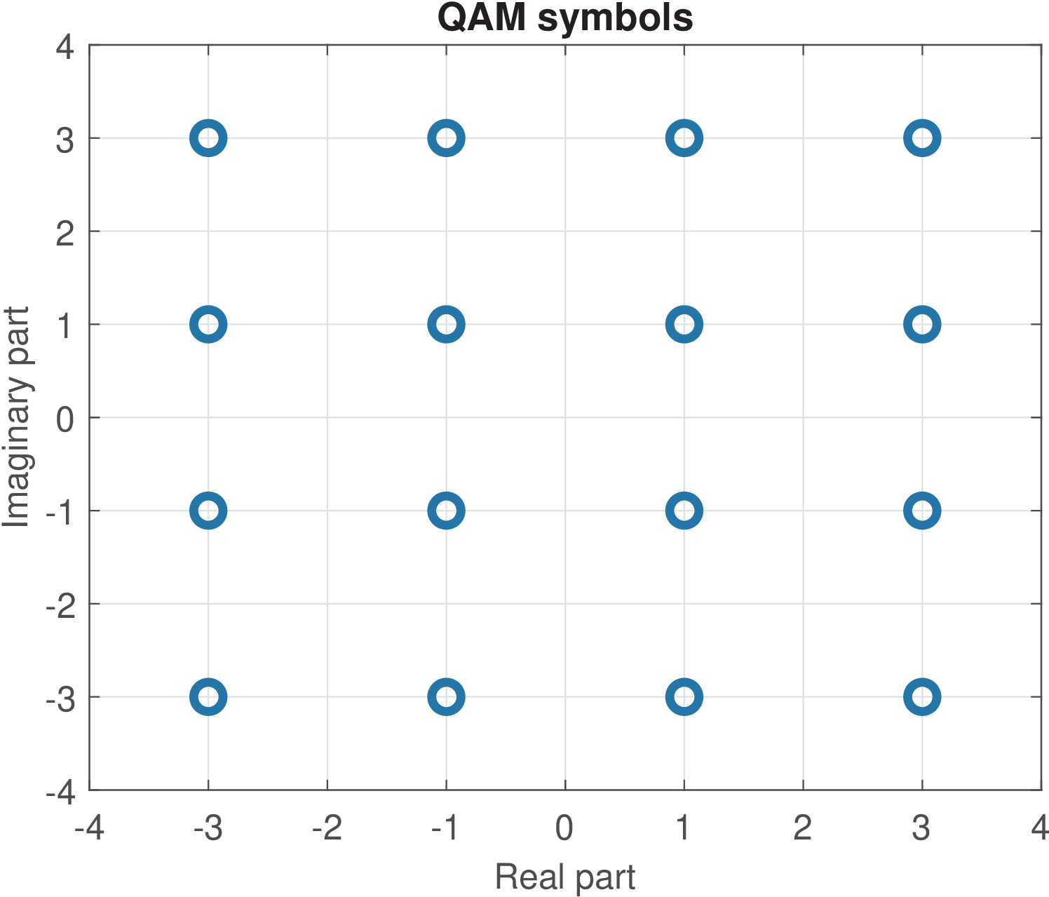
As indicated in Figure 2.24, the 16-QAM constellation can be interpreted as the Cartesian product of two 4-PAM constellations.

Constellations are useful when representing waveforms as vectors. This representation allows the establishment of several connections between signal and vector spaces. For example, the inner products between symbols (vectors in $ℝ^{D}$ ) can be made equal to the inner products between the continuous-time signals that represent these symbols, i. e.,

< m_{1}, m_{2} > = < s_{1} (t), s_{2} (t) >,

for the first and second symbols, for example.

It is convenient to represent signals by constellation symbols $m_{i}$ and abstract (or even ignore) the details of the respective waveforms $s_{i} (t)$ . For example, as long as the basis functions $φ_{j} (t)$ in Eq. (2.29) are orthonormal, the average energy of a signal constellation is invariant to the choice of these functions. In fact, a given constellation can be associated to several distinct sets of orthonormal basis functions with the same properties in terms of robustness to errors under AWGN, for example.

Figure 2.25 shows an example of generating a signal $s (t)$ using a 4-QAM constellation and $D = 2$ orthonormal basis functions. When $D = 2$ , it is mathematically convenient to represent the symbols $m = [m_{1}, m_{2}]$ as a complex-valued symbol $m = m_{1} + j m_{2}$ .

As depicted in Figure 2.25, the slicer organizes the bitstream and feeds the mapper with 2 bits at each iteration $n$ . The mapper uses a 4-QAM constellation to convert the binary input into symbols $m$ . For example, at iteration $n = 0$ the bits are “01”, which is mapped via the defined constellation to the symbol $1 + j$ . The real parcel (1 in this case) of this symbol multiplies $φ_{1} (t)$ while the imaginary part (also 1) multiplies $φ_{2} (t)$ . This way, the real and imaginary parcels of the complex-valued symbols $m$ multiply the corresponding basis function $φ_{j} (t), j = 1, 2$ , to create $s (t)$ . Note that $T_{sym}$ is the duration of each iteration $n$ .

Figure 2.25: Creating a signal using a 4-QAM constellation and $D = 2$ orthonormal basis functions.

2.12.3 Recovering the symbols via correlative decoding

Orthogonal basis allows inner products to recover the symbols

Inner products are key elements to represent waveforms as vectors, as discussed in Section D.3 and Appendix A.12.3. Given that the set ${φ_{j} (t)}$ of orthonormal basis functions used to generate the transmit waveform is known to the receiver, the symbol $m$ can be obtained using correlative decoding as indicated by Eq. (D.9).

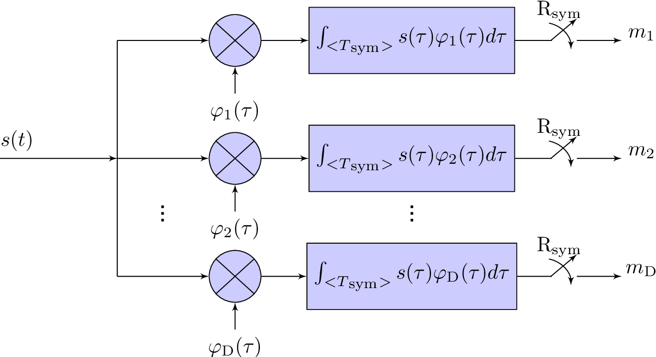
Figure 2.26: Correlative decoding, which when applied to $s (t)$ of Eq. (2.30) and properly sampled at its outputs, can recover the symbols $m_{i} = [m_{1}, \dots, m_{D}]$ .

Figure 2.26 depicts the correlative decoding process, which is capable of recovering the constellation symbols $m_{i}$ used to create $s (t)$ in Eq. (2.30). A clock synchronized with the symbol rate $R_{sym} = 1 ∕ T_{sym}$ is required to calculate inner products, each with a time interval $T_{sym}$ . Considering a given symbol, the process can be written in a simplified form as

m_{j} = < s (τ), φ_{j} (τ) > = \int_{< T_{sym} >} s (τ) φ_{j} (τ) dτ,

(2.32)

where $m_{j}$ is the $j$ -th element of the current symbol $m_{i}$ . The use of an inner product between signals as in Eq. (2.32) is analogous to its use between vectors, as discussed in Example A.1.

Example 2.7. Obtaining the symbols of a linear combination of basis functions. Using a procedure similar to Example A.1, consider that the transmitter uses $D = 3$ basis functions to embed the $n$ -th information symbol $m [n] = [3, - 5, 2]$ into a segment of the transmit waveform $s_{n} (t) = 3 φ_{1} (t) - 5 φ_{2} (t) + 2 φ_{3} (t)$ according to Eq. (2.29). Now the task is to recover the symbol $m [n] = [m_{1}, m_{2}, m_{3}]$ via the correlative decoder of Figure 2.26.

Assuming the received signal coincides with the transmitted $s (t)$ , to recover the first element $m_{1}$ of the $n$ -th symbol, the inner product between $s_{n} (t)$ and $φ_{1} (t)$ can be used as follows:

\begin{array}{l} m_{1} = ⟨ s_{n} (t), φ_{1} (t) ⟩ & = ⟨ 3 φ_{1} (t) - 5 φ_{2} (t) + 2 φ_{3} (t), φ_{1} (t) ⟩ \\ = 3 ⟨ φ_{1} (t), φ_{1} (t) ⟩ - 5 ⟨ φ_{2} (t), φ_{1} (t) ⟩ + 2 ⟨ φ_{3} (t), φ_{1} (t) ⟩ \\ = 3 \times 1 - 5 \times 0 + 2 \times 0 = 3, \end{array}

where the second step was obtained due to the linearity of an inner product and the third one due to the orthonormality of the basis functions. The other elements of $m [n]$ can be retrived via $m_{2} = ⟨ s_{n} (t), φ_{2} (t) ⟩$ and $m_{3} = ⟨ s_{n} (t), φ_{3} (t) ⟩$ , as suggested by Figure 2.26. $□$

The previous example assumed a single symbol, but a receiver has the more complicated task of dealing with a signal that represents a sequence of symbols. In practice, the receiver chooses a time instant $t_{0}$ (or a sample in discrete-time) called cursor, which serves as a time reference to the start of a symbol, and periodically makes a decision at a rate $1 ∕ T_{sym}$ . The cursor and baud rate may have to be continuously adjusted in a closed loop for tracking small variations.

Correlative decoding maximizes SNR when the channel is AWGN

When the channel is AWGN, correlative decoding achieves the optimum performance. A sketch of a proof to this is deferred to Section 4.3.8 and it will be based on the equivalence between correlative decoding and matched filtering.

In the sequel, the goal is to simply develop some intuition about how correlative decoding performs when the input signal is not the transmit signal $s (t)$ as in Figure 2.26, but a signal $r (t) = s (t) + ν (t)$ contaminated by noise $ν (t)$ . For that, it suffices to consider the transmission of a single symbol $m$ . For simplicity, it is assumed PAM with $D = 1$ and $φ_{1} (t) = p (t)$ being a shaping pulse with unitary energy.

As discussed in Section C.10, correlation is a measure of similarity. Because the receiver knows that the transmitted signal was composed by repeatedly scaling the shaping pulse $p (t)$ by symbol values, it is sensible to perform the correlation between the received signal $r (t)$ and the shaping pulse $p (t)$ itself. This way, when there is no noise ( $ν (t) = 0$ ) and $r (t) = mp (t)$ , the correlation is

⟨ r (t), p (t) ⟩ = m | | p (t) | |^{2} = m

(2.33)

More importantly, when AWGN is present and $r (t) = mp (t) + ν (t)$ , the correlation is

⟨ r (t), p (t) ⟩ = ⟨ mp (t), p (t) ⟩ + ⟨ ν (t), p (t) ⟩ = | | p (t) | |^{2} m + N = m + N,

(2.34)

where the random variable $N$ has variance $σ^{2} = N_{0} ∕ 2$ , as suggested by Eq. (F.48), which adopts a filtering notation instead of correlation. This is the minimum noise power that can be observed given the receiver architecture of Figure 2.26.

The noise parcel $N$ is uncorrelated with $m$ , such that the power of their sum in Eq. (2.34) is the sum of their individual powers. By definition, the power associated to parcel $m$ in Eq. (2.34) is the constellation energy ${\bar{E}}_{c} = 𝔼 [| m |^{2}]$ . Hence, the SNR at the AWGN output is

SNR = \frac{{\bar{E}}_{c}}{N_{0} ∕ 2},

(2.35)

because ${\bar{E}}_{c}$ and $N_{0} ∕ 2$ are the power of the discrete-time signals derived from the signal of interest $mp (t)$ and noise $ν (t)$ , respectively.

If the transmit pulse $p (t)$ does not have unitary energy, the correlative decoder can use a normalized version of $p (t)$ without any penalty in performance. In fact, any scaling at the receiver affects both the signal of interest and noise, such that the SNR is not altered, as will be discussed in Section 4.3.4. In contrast, scaling $p (t)$ at the transmitter can lead to a stronger signal of interest at the receiver and improve performance. Hence, to simplify the notation, it is convenient to assume unitary energy pulses and control the transmit power via the constellation energy $E_{c}$ .

2.12.4 Interpreting digital modulation as transforms

Correlative decoding has this name because the cross-correlation between the input signal $s (t)$ and each basis function $φ_{i} (t)$ is repeatedly calculated, as indicated in Figure 2.26. is similar to finding the coefficients using an inverse transform as discussed in the sequel.

It is useful to make the connection between modulation / demodulation and transforms. The correlative decoding of Figure 2.26 uses inner products that can be made equivalent to a transform $X = A^{H} x$ . In digital communications, one can interpret the generated “time-domain” signals $x$ (or $s (t)$ in the continuous-time case) as inverse transforms of a finite number of possible coefficient vectors $X$ .

When compared to other applications of transforms, the following characteristics of their use in digital communications are emphasized:

The number of basis functions is finite and relatively small (two, for example).
The transform matrices $A$ and its inverse are not square.
While some applications of transforms do not impose restrictions to the coefficient values, in the context of digital communication system, the transform coefficients $X$ are restricted to the finite set of symbols called constellation.
The basis are often real functions and $A^{H}$ is simply the transpose of $A$ such that the functions $φ (t)$ that appear in Figure 2.26 are used in both transmitter and receiver.

The following example uses QAM modulation to illustrate the analogy.

Example 2.8. QAM modulation interpreted as a transform. Assume a digital communication system uses simultaneously the amplitudes of a cosine and a sine to convey information to the receiver. Assume also that the possible amplitude values for both cosine and sine, are $- 3, - 1, 1, 3$ , corresponding to a 4-PAM for each of the two dimensions of the QAM. Assume also that in a discrete-time implementation, each message (or symbol) is represented by $S = 32$ samples and both sinusoids have a period of 8 samples. Hence, each symbol in time-domain is given by

x [n] = \sqrt{\frac{2}{S}} [A_{c} cos (\frac{2 π}{8} n) + A_{s} sin (\frac{2 π}{8} n)], n = 0, \dots, S - 1,

where $A_{c}$ and $A_{s}$ are the amplitudes of the cosine and sine, respectively, and the scaling factor $\sqrt{\frac{2}{S}}$ normalizes the basis functions to have unity energy (as in the DCT). Note that for each block of $S = 32$ samples there is a pair $(A_{c}, A_{s})$ . Because there are $M = 16$ possible pairs $(A_{c}, A_{s})$ , each symbol can carry $b = {log}_{2} 16 = 4$ bits.

In an analogy to block transforms, the amplitudes $A_{c}$ and $A_{s}$ play the role of the coefficients, and the transform matrix $A$ has dimension $S \times D$ , with $D = 2$ columns consisting of the cosine and sine samples. In this case the matrix transform is not square and a pseudoinverse should be adopted for mathematical consistency when obtaining the inverse of $A$ . In practice, given that the columns are orthonormal, the pseudoinverse of $A$ is $A^{H}$ . Hence, given a vector $x$ representing the samples of $x [n]$ , the coefficients $X = {[A_{c}, A_{s}]}^{T}$ can be obtained by $X = A^{H} x$ . Listing 2.15 illustrates the procedure.

Listing 2.15: MatlabOctaveCodeSnippets/snip_digi_comm_digital_mod_transf.m

1S=32;       %number of samples per symbol 
2Period=8;   %period of sinusoids 
3n=(0:S-1)'; %time index 
4%inverse matrix: 
5A=[cos(2*pi/Period*n) sin(2*pi/Period*n)]*sqrt(2/S); 
6innerProduct=sum(A(:,1).*A(:,2)) %are columns orthogonal? 
7if 1  %test two alternatives to obtain Ah from A 
8  Ah=A'; %the pseudoinverse is the Hermitian 
9else 
10  Ah=pinv(A); %equivalently, use pseudoinverse function 
11end 
12Ac=3; As=-1; 
13x=Ac*A(:,1)+As*A(:,2); %compose the signal in time domain 
14X=Ah*x  %demodulation at the receiver: recover amplitudes

It should be noted that the period of 8 samples was chosen such that $S = 32$ corresponds to an integer number of periods and the sinusoids are orthogonal. Try to use a period of 9 in the previous script and you will note that the original amplitudes cannot be perfectly recovered. Listing 2.22 provides another, and more complete, example of using transforms for correlative decoding. $□$