Baseband Line Codes

2.10 Baseband Line Codes

In this section, the PAM concept is expanded by varying the shaping pulse $p (t)$ to obtain digitally modulated signals in baseband, which are often called line codes. One important goal of this study is to show how the shaping pulse determines the signal PSD, which then should be compatible with the frequency response of the channel in which the signal is transmitted. This section assumes binary systems, but $M$ -ary versions of line codes are also used.

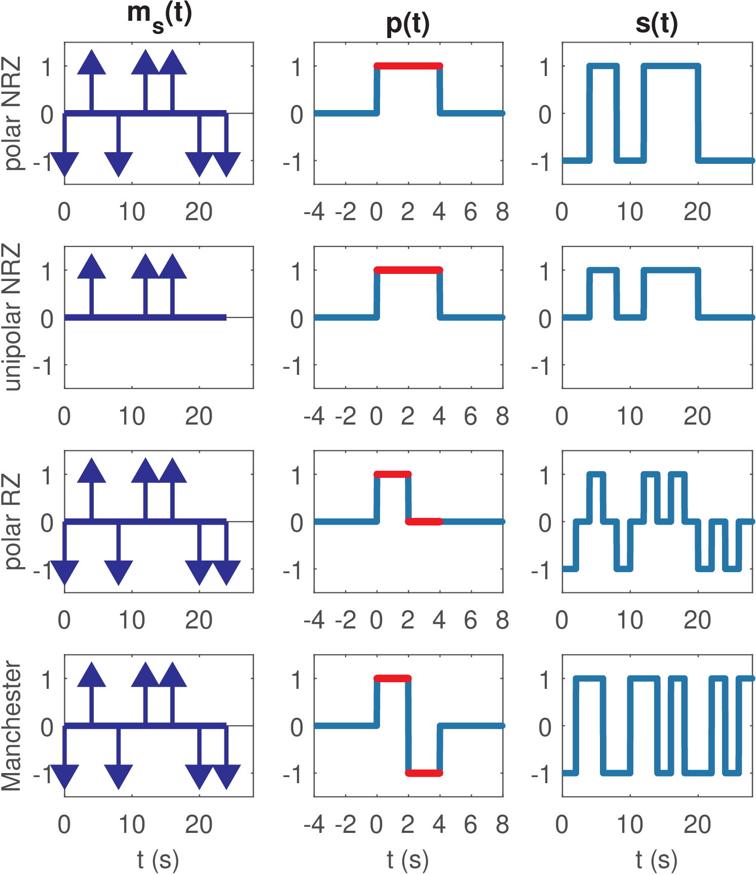
Figure 2.15 illustrates three line codes: polar NRZ, unipolar NRZ and polar RZ, all obtained by memoryless linear modulation according to Block (2.15). As mentioned, the term RZ (return to zero) is adopted when the pulse $p (t)$ goes to zero within its duration $T_{sym}$ . The terms polar and unipolar are used when the symbols $m_{i}$ are signed and unsigned (non-negative), respectively. The Manchester is a line code that uses polar symbols but a $p (t)$ with positive amplitude in half of $T_{sym}$ and a negative amplitude in the other half. It provides a more robust synchronization at the receiver than the NRZ codes. Consider a long sequence of the same bit 0 or 1, for example. It is easier to learn where a symbol starts when using Manchester when compared to a NRZ signal, which would correspond to a signal with constant amplitude in this case.

Figure 2.15: Polar NRZ, unipolar NRZ and polar RZ line codes. The symbol interval is $T_{sym} = 4$ s and the bit stream was [0 1 0 1 1 0 0].

The line codes in Figure 2.15 are memoryless. Two examples of line codes with memory are depicted in Figure 2.16: bipolar (also called pseudoternary and alternate mark inversion - AMI) and differential. The memoryless polar NRZ is included for convenience, because it provides a reference to interpret the other codes. The bipolar code is obtained by transmitting no pulse for bits 0 and pulses of alternating polarity for bits 1.

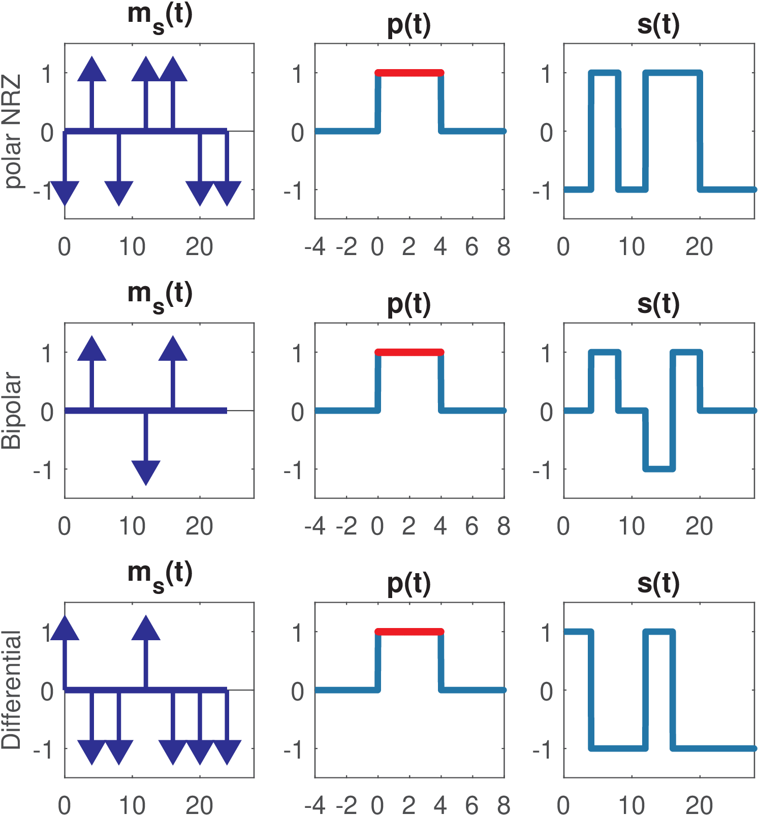
Figure 2.16: Line codes NRZ polar, bipolar and differential. The last two have memory. The symbol interval was $T_{sym} = 4$ s and the bit stream was [0 1 0 1 1 0 0] as in Figure 2.15. For the differential code, the initial bit was assumed equal to 1 and the differential bit stream was [1 0 0 1 0 0 0].

An important advantage of bipolar is that it contains no DC component even if a long string of 0’s or 1’s occur. Listing 2.12 illustrates the procedure for the bipolar code when generating its plot in Figure 2.16.

Listing 2.12: MatlabOctaveCodeSnippets/snip_digi_comm_bipolar_code.m

1bits=[0 1 0 1 1 0 0]; %bits to be transmitted 
2N=length(bits); %number of bits 
3m=zeros(1,N); %pre-allocate space for symbols 
4currentPolarity = 1;%assumption: positive polarity first 
5for i=1:N %loop over bits 
6    if bits(i)==1 
7        m(i)=currentPolarity; 
8        currentPolarity = -currentPolarity; %invert 
9    end %no need for "else": m(i) is initialized as zero 
10end

The differential line code in Figure 2.16 was generated with Listing 2.11, which was discussed in Section 2.9.3.

In summary, some considerations for selecting line codes (i. e., signaling schemes) are:

Power spectral density, particularly its value at 0 Hz (DC level) and bandwidth;
Ease of clock signal recovery for symbol synchronization;
Error detection properties.