Concepts and Elements of a Digital Communication System

2.3 Concepts and Elements of a Digital Communication System

2.3.1 Block diagram of a digital communication system

Figure 2.1 is a block diagram representing a generic Tx of a digital communication system. The overall task of the Tx is to convert the information into an analog waveform $s (t)$ that is suitable for transmission over a channel $h_{c} (t)$ (not shown).

Figure 2.1: Block diagram of a generic transmitter.

Figure 2.2 illustrates a generic⁴ receiver.

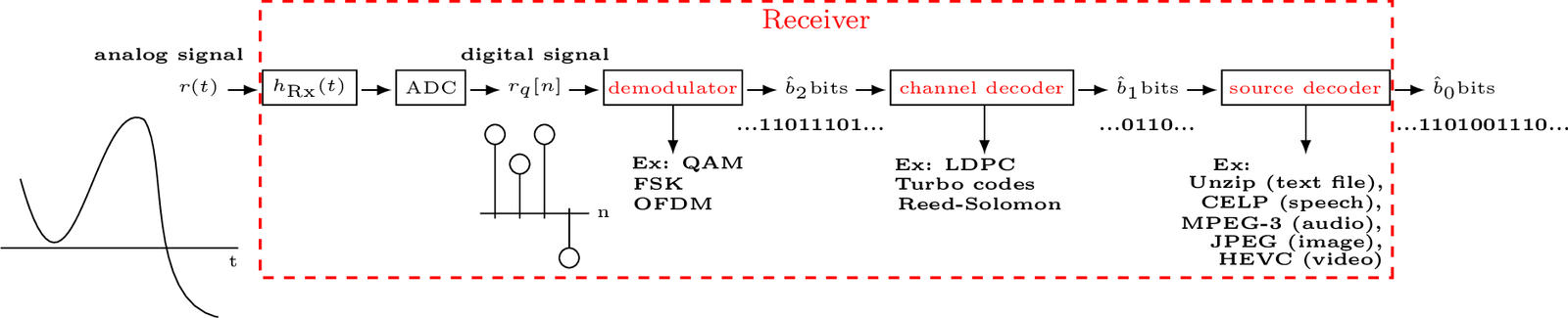
Figure 2.2: Block diagram of a generic receiver.

In practice, the analog LTI system denoted by its impulse response $h_{Tx} (t)$ is responsible for filtering and amplification. For example, wireless systems use power amplifiers before the transmitting antennas to achieve the required coverage area. Another role played by $h_{Tx} (t)$ is to perform the D/A “reconstruction” filtering. All digital signals are periodic and an analog filter should be used to eliminate undesired replicas, as exemplified in Figure E.18, and keep only the spectrum frequency range that conveys information. Similarly, the receiver also uses an analog LTI system $h_{}$

Rx(t) $t o p e r f o r m a n t i - a l i a s i n g f i l t e r i n g a n d r e d u c e t h e n o i s e p o w e r b e f o r e t h e A ∕ D c o n v e r s i o n . T h e a n a l o g s y s t e m s$ h_Tx(t) $a n d$ h_Rx(t) $a r e c l e a r l y i m p o r t a n t b u t t h e y a r e a s s u m e d t o b e i d e a l f i l t e r s i n m o s t d i g i t a l c o m m u n i c a t i o n s l i t e r a t u r e .$

Most of the discussion in this text is concentrated on the digital part of the transmitter (i. e., on how to generate $s_{q} [n]$ ) and, later, at the digital part of the receiver (how to interpret $r_{q} [n]$ after A/D conversion).

2.3.2 Number of bits per second can vary over the stages

Let us assume that, in Figure 2.1 and Figure 2.2, the bitstreams $b_{i}$ and ${\hat{b}}_{i}$ , for $i = 0, 1, 2$ have a finite length denoted as $N {b_{i}}$ and $N {{\hat{b}}_{i}}$ , respectively. Ideally, the number $N {b_{i}}$ of bits at each stage of the Tx in Figure 2.1 is the same as its counterpart $N {{\hat{b}}_{i}}$ at the Rx in Figure 2.2. In practice, however, there are situations that may lead to $N {{\hat{b}}_{i}} \neq N {b_{i}}$ . For example, most video codecs, such as MPEG-4, use a variable rate bitstream, i. e., the instantaneous rate (number of bits per second) varies according to the scene contents. Transmission errors can potentially lead to $N {b_{0}} \neq N {{\hat{b}}_{0}}$ . Another example is that synchronization errors can imply in $N {b_{2}} \neq N {{\hat{b}}_{2}}$ .

2.3.3 Source coding

The number $N {b_{0}}$ of bits (ADC output) is typically high and source coding is the stage that tries to eliminate redundancy such that $N {b_{1}} < N {b_{0}}$ . When one compresses a file with softwares such as Winzip, Winrar, gzip, etc., it is basically using source coding techniques. An example of the importance of the source coder is the much smaller size of an image in the PNG format when compared to the plain bitmap (BMP) formats. Both PNG and BMP are examples of lossless formats, meaning that the process of coding and decoding does not change the original information. When a lossy coding technique can be used, the compression ratio is significantly larger. This is the main reason for the popularity of lossy file formats such as DivX, MP3 and JPEG to store video, audio and images, respectively. Source coding is a rather specialized area and is the subject of many textbooks.

2.3.4 Channel coding

It may sound exquisite, but after the effort of the source encoder to eliminate redundancy, the next block, the channel coder, adds redundancy such that $N {b_{2}} > N {b_{1}}$ in Figure 2.1. Different from the redundancy in the original binary source, this controlled redundancy allows the detection and correction of transmission errors.

There are many channel coders (e. g., Reed-Solomon, LDPC, etc.) and here the simple repetition code is used as an example: if for each bit $x \in {0, 1}$ to be transmitted, a channel coder adds two extra copies of this bit to form a triple $x x x$ , it is intuitive that the receiver could make decisions based on the majority of bits in each triple. For example, 010 could be interpreted as a transmitted 0 that suffered an error in one of its three coded bits. This way, the receiver could detect and correct the occurrence of a single bit error at the expense of an overhead of two extra bits per information bit.

Among the schemes for channel coding, forward error correction (FEC) is widely used because it does not depend on feedback from the receiver. One important parameter of a FEC is its code rate, which is the proportion of useful (that are carrying information bits), often denoted as $k ∕ n$ . In this case, for $k$ bits of information, the encoder generates $n - k$ bits of redundancy and outputs $n$ bits. Hence, the net bitrate (useful information) is the fraction $k ∕ n$ of the gross bitrate.

2.3.5 Modulation

The digital modulator block typically does not change the number of bits used to represent information,⁵ i. e., $s [n]$ corresponds to $N {b_{2}}$ bits. As mentioned in Section 1.5, the role of modulation is to create waveforms that can be properly transmitted through the channel and interpreted at the receiver.

2.3.6 Demodulation

Demodulation is the (eventually complicated) process of converting the received waveform $r (t)$ into bits.

Result 2.1. Advanced: Definition of demodulation. As for the term “modulation”, this definition of demodulation is not universal given that the jargon in telecommunications is far from consensual. For example, some authors prefer to define demodulation as synonymous of frequency downconversion. The more general definition is adopted here and demodulation is considered the whole process, which may include obtaining baseband pulses from the received waveform $r (t)$ , and a subsequent decision or detection process being responsible for converting these pulses into bits in digital communications. There are advantages in adopting this more general definition of demodulation: for example, in Matlab/Octave, functions such as pamdemod simply perform the “detection” process, which would be confusing under the light of a definition in which demodulation is restricted to frequency downconversion and does not include detection. $□$

Figure 2.3 provides an example of a baseband demodulator. In this case there is no need for downconversion because the signal of interest is already centered at DC. The timing recovery block uses analog processing (e. g., a circuit with a PLL that tracks a sinusoid extracted from $r (t)$ as discussed in Section 4.11.3) to drive the sampler and obtain $y [n]$ sampled at $R_{sym}$ . The detector⁶ finds the estimated symbol $\hat{m} [n]$ that best represents $y [n]$ given the constellation and decision criterion (e. g., maximum likelihood, as discussed in Section 5.3). The demapper simply converts each constellation symbol to its respective binary representation.

Figure 2.3: Example of baseband demodulator (which in this case implements a complete receiver).

The demodulator in Figure 2.3 is a complete receiver, which can be made more sophisticated by the inclusion of channel (de)coding, etc. In fact, there are several alternatives for implementing a receiver with similar functionality. For example, the signal $r (t)$ can be digitized at a sampling rate $F_{s}$ and all timing recovery implemented in the digital domain.

The nomenclature in Figure 2.3 may vary: the detector and demapper are called, respectively, slicer and decoder in some textbooks. The various architectures and definitions found in the literature can be confusing. It is important to have the Tx / Rx blocks clearly defined according to a consistent nomenclature. Figure 2.3 informs the one adopted in this text.

With demodulation defined as the whole process of interpreting $r (t)$ as bits, the demodulator performs at the receiver, operations that are the inverse of the corresponding ones at the modulator (e. g., the demapper inverts the mapper) and some extra ones. The receiver is typically more computationally complex than the transmitter. Some of the main actions performed by a demodulator are:

synchronization;
frequency downconversion;
detection.

with frequency downconversion typically depending on the synchronization, as explained in the sequel.

2.3.7 Synchronization and Coherent Demodulation

The two main tasks of a synchronizer are timing and carrier recovery. Timing or symbol recovery is the process of choosing the best time instants to sample a waveform to get good estimates $\hat{m} [n]$ of the transmitted symbols $m_{i}$ . Timing recovery is a requirement of virtually all digital communication systems. In some cases a clock signal is transmitted apart from the information signal, and in other cases the timing information is embedded or should be extracted from the information signal itself.

Among the systems that use upconversion, some require estimating the carrier at the Rx (recovery) to perform coherent demodulation while others adopt noncoherent demodulation. Coherent, also called synchronous,⁷ demodulation means that the receiver aims at regenerating both the carrier frequency $f_{c}$ and phase $ϕ_{c}$ to perform frequency downconversion. After estimating its parameters and recovering the carrier $ĉ (t)$ , the receiver typically implements the downconversion by multiplying the received signal and $ĉ (t)$ and then filtering.

An example of a noncoherent system is the one that uses amplitude modulation (AM) and recovers the information based on the envelope of the received signal as discussed in Application 1.2. Coherent systems are typically more complex but have a better performance than their noncoherent counterparts. In optical communications, for example, the recent advances in electronics have allowed ADCs with $F_{s}$ of the order of GHz and fast enough to digitize the signal obtained from the received electrical field. This has enabled many new coherent demodulation schemes and the adoption of digital signal processing techniques to compensate impairments such as nonlinearities.

But it is not trivial to keep the Tx and Rx in synchronism. Their clock generators and oscillators are set to the same nominal values but, due to circuit imperfections, temperature variations, etc., the signals at the Rx can drift with respect to the ones at the Tx. The accuracies of clock generators and oscillators are specified in parts per million (ppm) but, even when they are very accurate, closed-loop adaptive techniques such as phase-locked loops (PLLs) are used to continuously track the Tx signals at the receiver. Application 1.5 discusses synchronization in GSM cellular networks.

2.3.8 Digital signals in digital communications

It is possible to implement a digital communication system using analog processing, but it is much more common to use digital signal processing. Hence, it is assumed here that the transmitter creates a digital signal $s_{q} [n]$ , which is converted to an analog waveform via D/A conversion. This waveform is processed by an analog LTI system with impulse response $h_{Tx} (t)$ (the transmitter filter) to generate $s (t)$ , which is sent through the channel as depicted below

\begin{array}{l} bits \to Digital Tx \to s_{q} [n] \to DAC \to h_{Tx}(t) \to s (t) . & (2.2) \end{array}

In spite of $s_{q} [n]$ being a digital signal, it is common to deemphasize the importance of the fact that its amplitude is discrete and represent it as a discrete-time signal $s [n]$ . Hence, the subscript $q$ in $s_{q} [n]$ is omitted hereafter.

2.3.9 Bit and symbol rates

In general, the bit rate $R$ (expressed in bits per second or bps) is

R = R_{sym} b,

where

b = {log}_{2} M

is the number of bits per symbol. Only for the case of a binary system, in which $b = 1$ , one has $R = R_{sym}$ .

Example 2.1. Distinction of bit and symbol rates. For example, assume that a digital system transmits 100 symbols per second ( $R_{sym} = 100$ bauds), with each symbol obtained from an alphabet with $M = 256$ symbols. Because $b = {log}_{2} M = 8$ bits, the rate is $R = R_{sym} b = 100 \times 8 = 800$ bps. $□$

2.3.10 Error rates: BER, SER and BLER

While analog communication systems try to preserve the waveform across the communication channel, the adoption of a finite set of waveforms allows the construction of digital communication systems that do not need to aim at reproducing the original waveform at the receiver. Hence, a digital communication system can be assessed via figures of merit that take into account that the goal is to transmit the bits, as explicitly represented in

bits \to Transmitter (Tx) \to s (t) \to Channel \to r (t) \to Receiver (Rx) \to \hat{bits} .

The symbol error rate (SER), denoted by $P_{e}$ , corresponds to the fraction of transmitted symbols that were wrongly recovered at the receiver. Similarly, the bit error rate (BER) is denoted by $P_{b}$ and corresponds to the fraction of transmitted bits that were wrongly recovered at the receiver. For example, in a 4-PAM (pulse-amplitude modulation) system ( $b = 2$ bits per symbol), the transmitted bits, corresponding to four symbols, are [01 11 11 00] and the received symbols are [01 00 10 00]. In this case, the second and third symbols have errors, and $P_{e} = 2 ∕ 4 = 0.5$ . The three wrong bits correspond to $P_{b} = 3 ∕ 8 = 0.375$ . Both SER and BER are defined here with the implicit assumption that the number of received symbols and bits, respectively, is equal to the number of transmitted symbols and bits. In practice these numbers may differ.

Note that

P_{b} \leq P_{e},

(2.3)

i. e., the BER is upper bounded by the SER. Only for binary systems or when all bits are wrong for every symbol error, one has $P_{b} = P_{e}$ . In fact, when a Gray code is used, in which neighboring symbols differ by a single bit, and the errors are always caused by a symbol being mistaken by one of its neighbors, one has

P_{b} = \frac{P_{e}}{b} .

(2.4)

Eq. (2.4) is the best possible $P_{b}$ for a given $P_{e}$ and combined with Eq. (2.3) leads to

\frac{P_{e}}{b} \leq P_{b} \leq P_{e} .

(2.5)

Changing the previous example to have the received bits as [01 01 10 00], the new BER would be $P_{b} = 2 ∕ 8 = 0.25 = P_{e} ∕ b$ .

In case the required information ( $p (i)$ , $P_{e} (j | i)$ , $n_{b} (i, j)$ ) is available, $P_{b}$ can be calculated by

P_{b} = \frac{1}{b} \sum_{i = 1}^{M} \sum_{j, j \neq i} p (i) P_{e} (j | i) n_{b} (i, j),

where $p (i)$ is the a priori probability of symbol $m_{i}$ , $P_{e} (j | i)$ is the probability of incorrectly choosing $m_{j}$ when $m_{i}$ was transmitted and $n_{b} (i, j)$ is the number of bits by which the symbols $m_{i}$ and $m_{j}$ differ.

In commercial communication systems, information is organized into frames or blocks. For example, LTE and 5G define a transport block as a sequence of bits that includes not only the payload but also an error detection code (specifically a CRC - cyclic redundancy check), which enables the receiver to detect whether the block was received with errors. This mechanism allows the calculation of the block error rate (BLER), defined as the ratio of the number of erroneously received blocks to the total number of transmitted blocks. Additionally, the presence of the CRC enables the receiver to request the retransmission of any block detected as erroneous. Rather than aiming for a BLER of zero, most wireless systems adopt a target of $BLER = 10 %$ , which reflects a trade-off: maximize throughput and reduce retransmissions while maintaining acceptable levels of reliability.

⁴ The diagrams of Figure 2.1 and Figure 2.2 are just examples. There are digital communication systems that do not use a source coder (also called encoder), for example, or do not include an ADC.

⁵ There are modulation techniques, such as trellis modulation that incorporate channel coding [PS07].

⁶ Some authors call this block “slicer” instead of detector, but here slicer is the process of chopping a bitstream to feed the mapper, as illustrated in Figure 2.25.

⁷ Both words, synchronous and coherent have other meanings in telecommunications as, for example, in synchronous digital hierarchy (SDH).