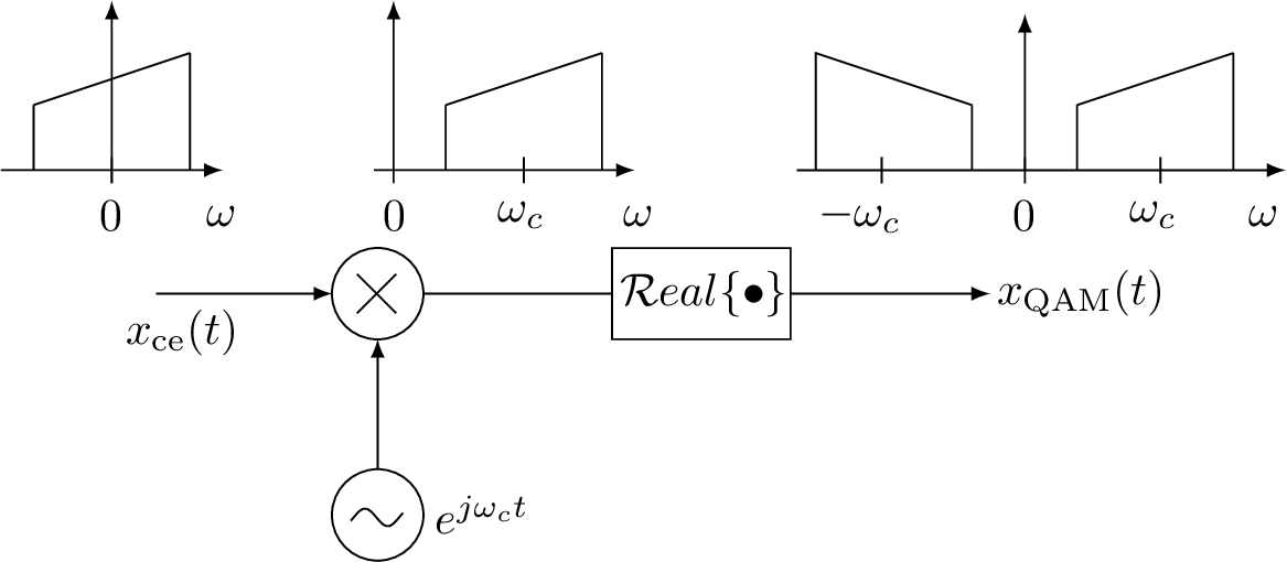
Using the complex-valued signals notation, the upconversion to generate the QAM signal can then be represented by a complex exponential and the $Real\{\cdot \}$ operation to extract the real part of the time-domain signal:

= Real { [x_i(t)- jx_q(t)] [cos ⁡ (ωct) + jsin ⁡ (ωct)]}

= x_i(t) cos ⁡ (ωct) + xq(t)sin ⁡ (ωct)(3.4)

which gives the same result as Eq. (3.2). Figure 3.5 illustrates the procedure.

To understand the spectra depicted in Figure 3.5, it is useful to interpret Eq. (3.4) in frequency domain. For this task, it is convenient to recall that the real part of a complex number $c$ can be obtained by $Real\{c\}=0.5(c+c^{\ast })$ and that $F\{x^{\ast }(t)\}=X^{\ast }(-\omega )$. Applying these two results to Eq. (3.4) leads to

= F{ 0.5 (x

ce(t) e^j ωct + x

ce^*(t) e^-j ωct)}

= 0.5 (F{x

ce(t) e^j ωct} + F{x

ce^*(t) e^-j ωct})

= 0.5 (Xce(ω − ωc) + Xce∗(−ω − ωc)).(3.5)

Note from Eq. (3.5) that the real and imaginary parts of $X_{\mathrm{\text{QAM}}}(\omega )$ are the even and odd parcels of the corresponding parts of $X_{\mathrm{\text{ce}}}(\omega )$. This implies, as expected, that $X_{\mathrm{\text{QAM}}}(\omega )$ has Hermitian symmetry given that $x_{\mathrm{\text{QAM}}}(t)$ is real-valued.

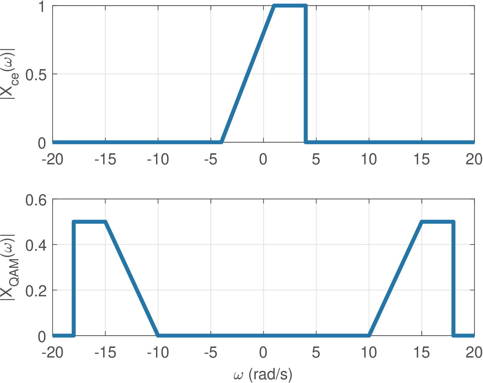
To provide more details on the spectra depicted in Figure 3.5, Figure 3.6 represents pictorially the spectrum magnitude $|X_{}$

ce(f)|$ofacomplexenvelopeobtainedfromrealsignals$x_i(t)$and$x_q(t)$.Notethatthe$X_ce(f)$doesnotpresenttheHermitiansymmetrybecause$x_ce(t)$iscomplex.Incontrast,theQAMsignalisrealand$X_QAM(f)$presentsthecorrespondingsymmetrywiththeversionsof$|X_ce(f)|$scaledbyhalf.$

The complex notation also allows to represent a QAM symbol $m=m_i-j{m}_q$, where $m_i$ and $m_j$ are two PAM symbols. The generation of the QAM signal is similar to the process used for a PAM signal: upsampling followed by convolution with a shaping pulse. Listing 3.3 illustrates the process, which takes advantage of the capability of Matlab/Octave to deal with complex-valued signals (filter, convolve, etc.). The adopted shaping pulse is a “raised cosine”, which will be discussed in Section 4.5.

1%generate QAM signal centered at Fs/4 
2M=16; %number of symbols 
3constellat=ak_qamSquareConstellation(M); %QAM const. 
4S=1000; %number of symbols 
5ind=floor(M*rand(1,S)); %indices 
6qamSymbols=constellat(ind+1); %sequence of random symbols 
7L=8; %oversampling factor 
8x=zeros(1,S*L); %pre-allocate space 
9x(1:L:end)=qamSymbols; %complete upsampling operation 
10p=ak_rcosine(1,L,'fir/normal',0.5,10); %raised cosine r=0.5 
11yce=conv(p,x); %complex env.: convolution by shaping pulse 
12%modulate by carrier at pi/2 rad that corresponds to Fs/4 
13n=0:length(yce)-1; %"time" axis 
14z=real(yce .* exp(j*pi/2*n)); %transmitted signal
  

The complex envelope was previously defined as $x_{\mathrm{\text{ce}}}(t)=x_i(t)-j{x}_q(t)$ because $Real\{x_{\mathrm{\text{ce}}}(t)e^{j{\omega }_{c}t}\}$ should lead to Eq. (3.2). Sometimes slightly different definitions are assumed: the summation in Eq. (3.2) is modified to a subtraction:

such that the complex envelope is defined with a summation:

in order to continue having $x_{\mathrm{\text{QAM}}}(t)=Real\{x_{\mathrm{\text{ce}}}(t)e^{j{\omega }_{c}t}\}$. The alternative Eq. (3.6) suggests defining a QAM symbol as $m=m_i+j{m}_q$ and will be used hereafter. In this case, the QAM generation of Figure 3.3 multiplies $x_q(t)$ by $-\text{sin}<!--FUNCTION\; APPLICATION-->(\cdot )$ instead of $\text{sin}<!--FUNCTION\; APPLICATION-->(\cdot )$. These latter definitions are assumed hereafter.

Figure 3.6 uses Fourier transforms, but similar result holds for PSDs. In fact, it can be inferred¹ from Eq. (F.34) that the average power $P_{\mathrm{\text{QAM}}}=𝔼[|x_{\mathrm{\text{QAM}}}(t){|}^2]$ of the real bandpass signal $x_{\mathrm{\text{QAM}}}(t)$ differs from the average power $P_{}$

ce = E[|x_ce(t)|^2]$of$x_ce(t) $byafactorof2,suchthat$

This is valid not only for QAM but for other bandpass signals obtained by upconverting a complex envelope. The factor of 2 also appears when modeling bandpass noise (or random signals, in general), which guarantees that signal to noise ratios are the same when representing bandpass signals by their corresponding lowpass complex envelopes.