4.7  Eye Diagrams

An eye diagram is used to observe the impact of noise and, especially, of ISI. The received signal is divided into segments of equal sizes. All the signal segments are plotted in the same figure, with persistence (e. g., using the command hold on on Matlab/Octave) so that they are overlapping. The length of the section should be a multiple of $T_{\mathrm{\text{sym}}}$.

The Listing 4.7 can be used to observe the incremental composition of an eye diagram for a 4-PAM modulation.

1%Generates a 4-PAM eye-diagram with a pulse as p[n] 
2N = 100; %Number of symbols 
3a = [-3 -1 1 3]; % Symbol alphabet 
4ind = floor(4*rand(N,1)) + 1;  %Integers between 1 and 4 
5pam = a(ind); % Generate 4-PAM symbol sequence 
6L = 3; % Oversampling factor 
7p = ones(1,L); %use a square pulse as shaping pulse 
8pams = zeros(size(1:L*N)); %pre-allocate space 
9pams(1:L:L*N) = pam; %sequence {a1 0 0 a2 0 0 a3 ...} 
10xn = filter(p,1,pams); % Pulse shaping filtering 
11increment = 3*L; %Number of samples to be shown 
12firstSample=1; %First sample to be shown 
13hold on; %Make the plots superimpose each other 
14lastSample = length(xn) - increment; %Last sample 
15abscissa = 0:increment-1; %Create a fixed x-axis 
16for i=firstSample:increment:lastSample 
17    segment = xn(i:i+increment-1) %show values 
18    plot(abscissa,segment,'bx-'); %plot these values 
19    pause %wait the user to observe the diagram formation 
20end

(a)

(b)

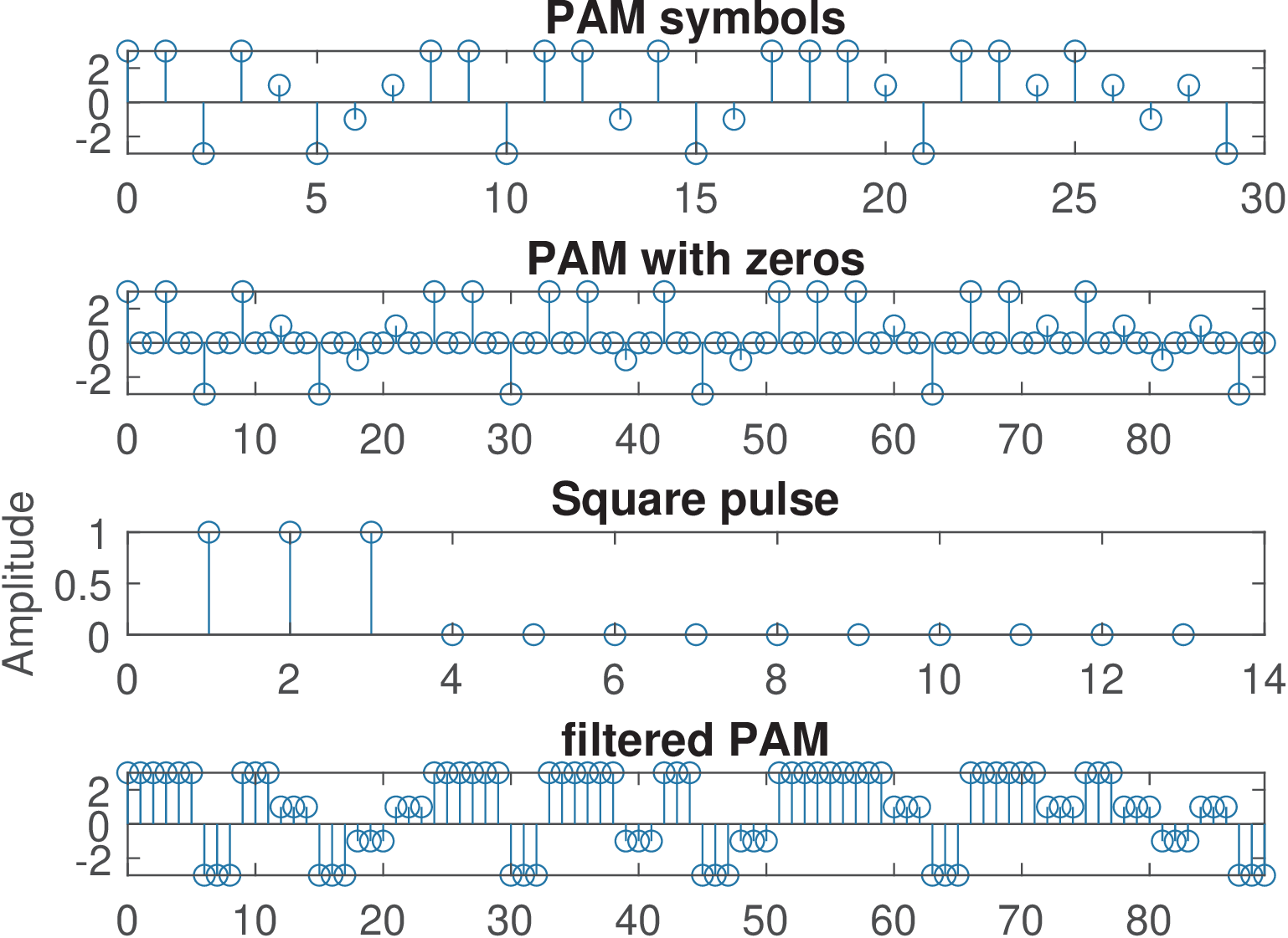
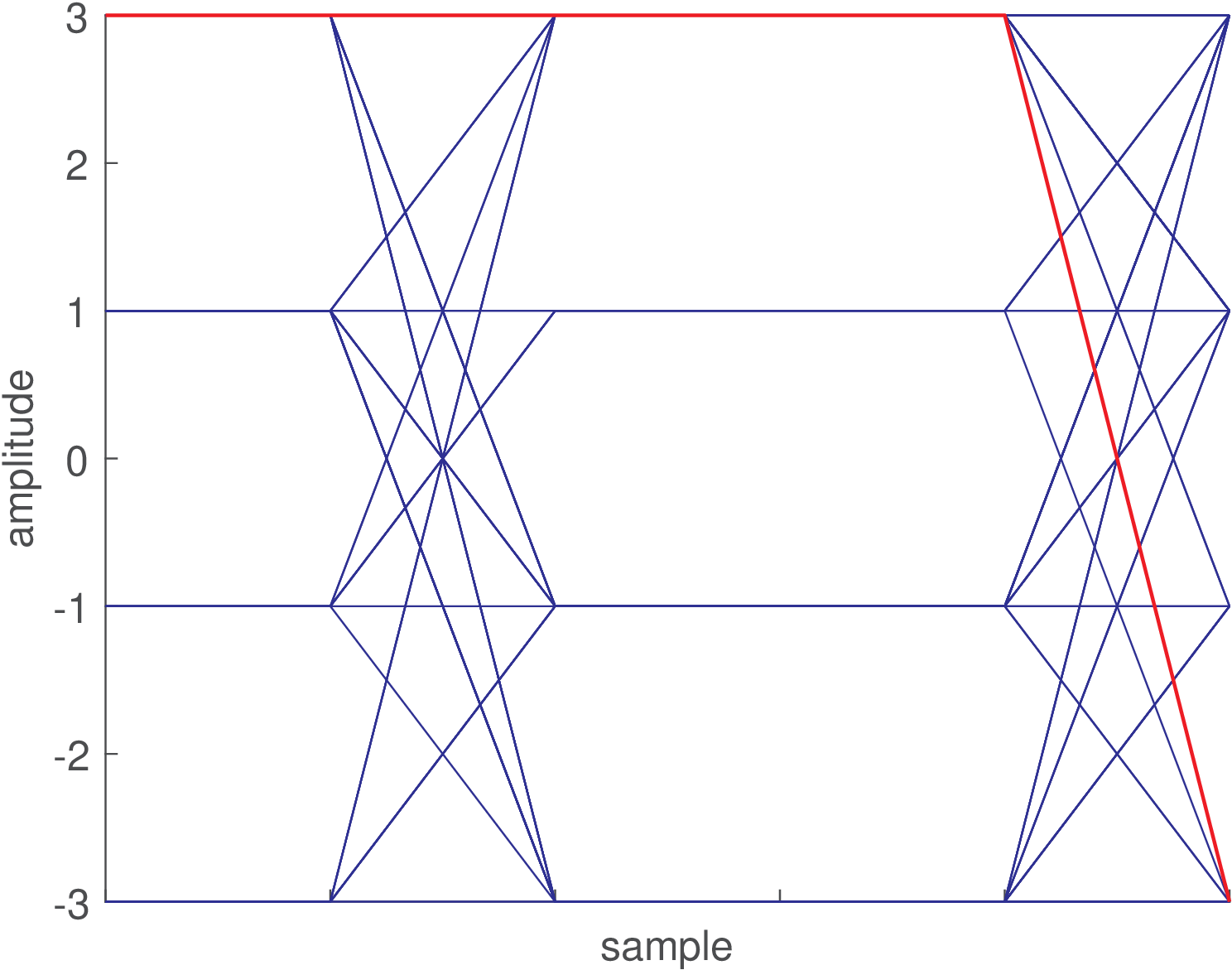
Figure 4.33 exemplifies an eye diagram generated with a code similar to Listing 4.7 and using a square wave as shaping pulse. The shaping pulse has three non-zero samples and the oversampling is $L\; =\; 3$. The time range of this diagram is $5T_s$, which corresponds to six samples as identified by the location of the ’x’ marks. Few modifications were done in Listing 4.7: the variable increment was decreased from $3L$ to $2L$ and firstSample was made equal to 2 to better centralize the diagram. Only 100 symbols were used to make easier tracking the construction of this diagram. The first segment (related to the first three symbols) of this diagram is identified with red circles. In this case, as can be seen in Figure 4.33(a), the first three symbols are $3,3$ and $-\; 3$. The eye diagram starts with the second sample of the first symbol (firstSample=2) and its first segment ends with the first sample of the symbol $-\; 3$.

(a)

(b)

(a)

(b)

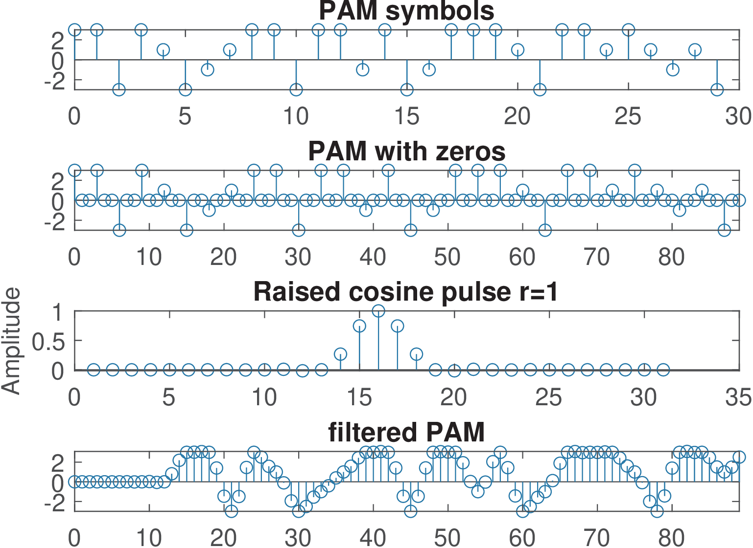
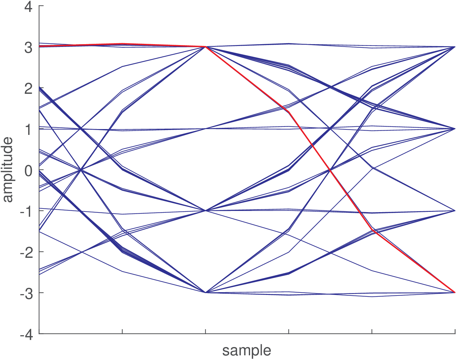
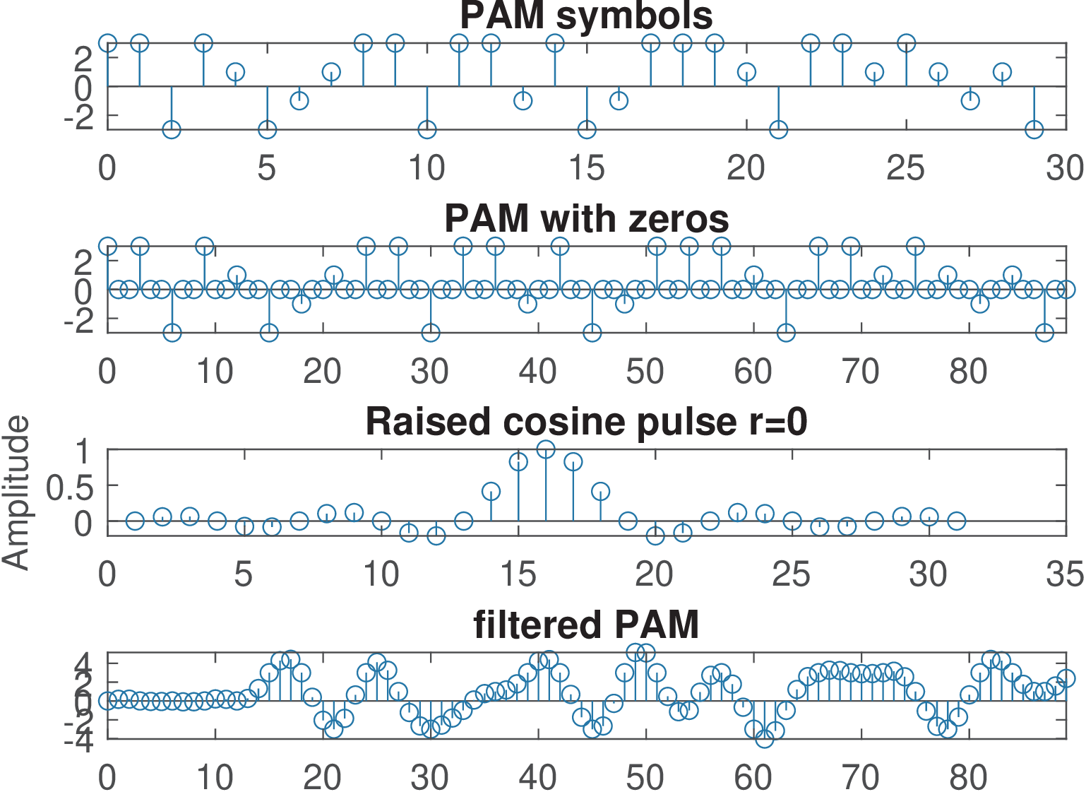
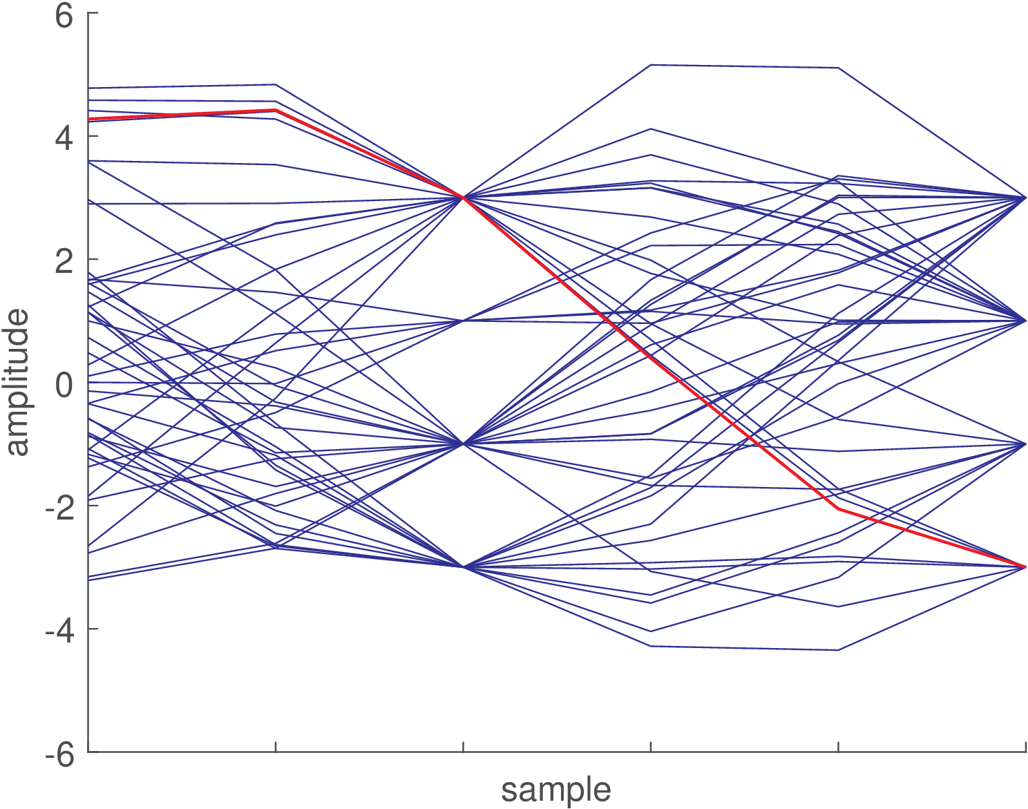
Figure 4.34 and Figure 4.35 use raised cosines with $r\; =\; 1$ and $r\; =\; 0$, respectively, and were generated using the same data as Figure 4.33. Contrasting the three figures, it can be noted that, when using a raised cosine, the transmitted value is perfectly recovered only at the correct sample instants. For example, while all three samples corresponding to the second transmitted symbol (equal to $+\; 3$) are the same in Figure 4.33, this value $+\; 3$ is observed only at the proper sample instant in Figure 4.34 and Figure 4.35. Therefore, eye diagrams indicate what happens when there is a synchronization error at the receiver with respect to the correct moment to extract a symbol. The horizontal opening of the eye diagram indicates the robustness of the system to eventual synchronization errors or errors in the so-called timing phase. When comparing Figure 4.34 and Figure 4.35, one can see that a raised cosine with $r\; =\; 1$ consumes twice the bandwidth of a raised cosine with $r\; =\; 0$, but the former is more robust against timing phase errors.

In summary, shaping pulses as the one used in Figure 4.33 are very effective against synchronization errors but may consume too much bandwidth, while the the roll-off factor $r$ of raised cosines allows to trade off bandwidth and complexity of the synchronization block at the receiver. Another interpretation is that the slope of the inside eye lid indicates the sensitivity to jitter (variations with respect to the assumed periodicity) in the timing phase.

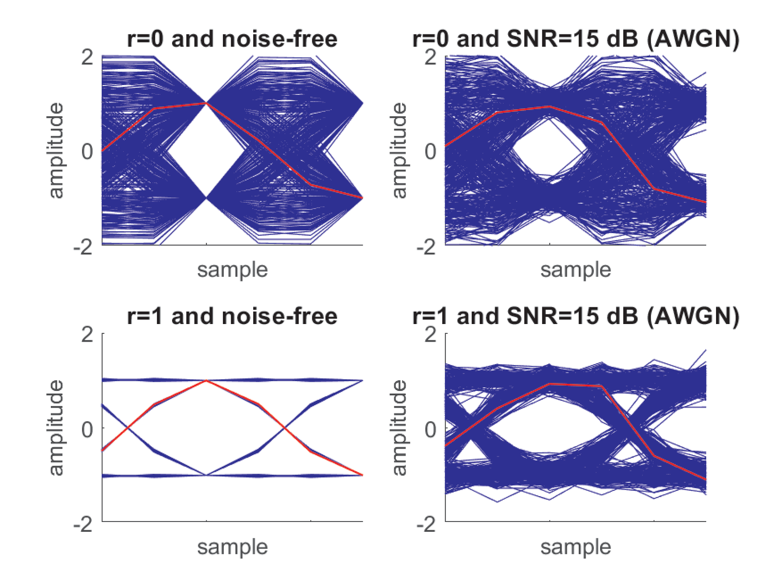
Besides synchronization, an eye diagram is also useful to infer about the noise at the receiver. Figure 4.36 uses binary transmission (2-PAM with symbols $\pm \; 1$), $L\; =\; 3$ and raised cosines with $r\; =\; 0$ and $r\; =\; 1$ under two scenarios: AWGN with 15 dB of SNR and noise-free transmission. It can be noted that the additive noise impacts the vertical opening of the eye and, even at the proper sampling instants, the received signal is not perfectly recovered as in the noise-free transmission.

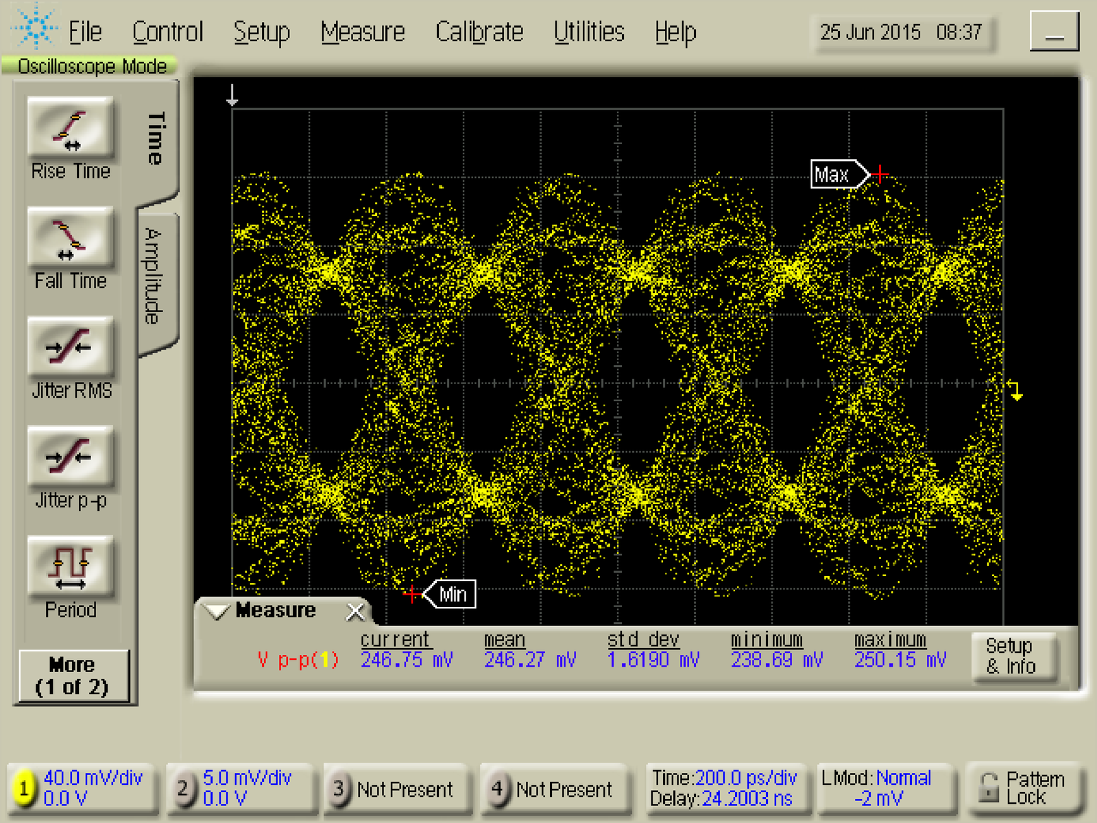
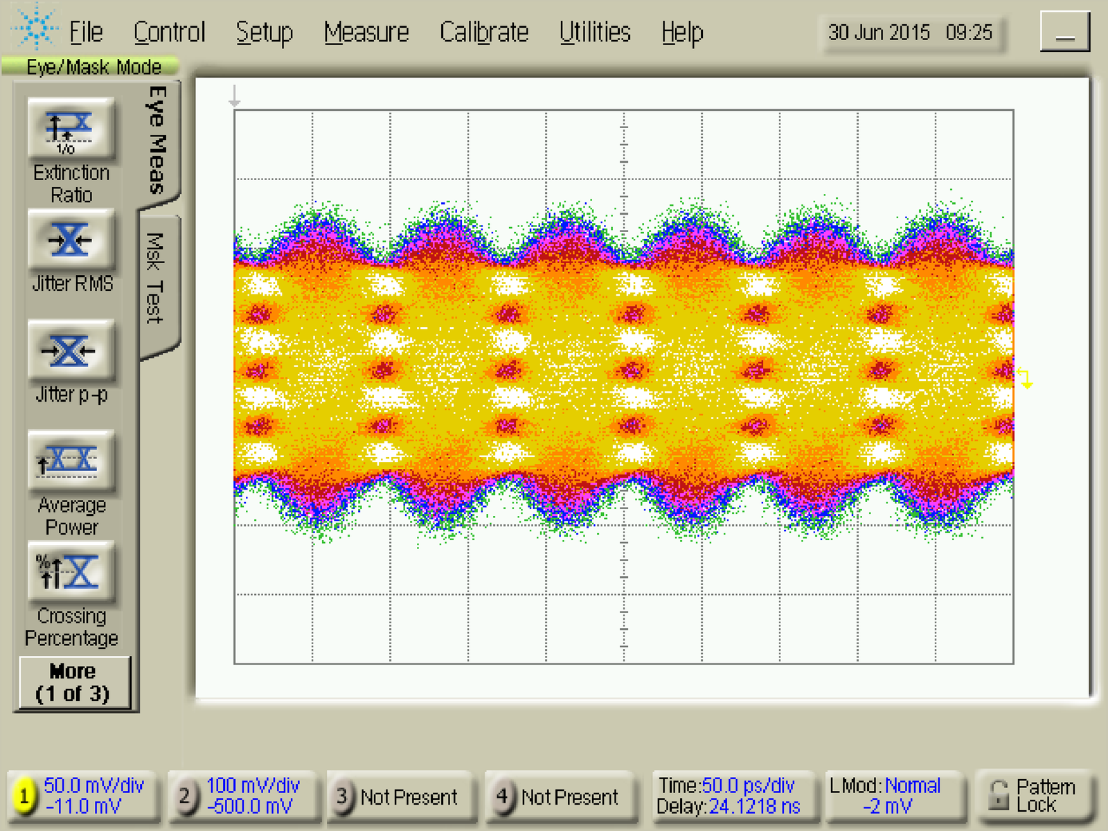
Figure 4.37 and Figure 4.38 provide examples of eye diagrams from actual measurements.