Channel Models

4.2 Channel Models

The WGN model is based on two assumptions: a) the noise amplitudes are distributed according to a Gaussian and b) the noise PSD is “white”, i. e., its power is equally distributed over all frequencies such that the PSD is flat. Gaussian does not imply white nor vice-versa. It is possible to have a Poisson white noise, for example, or a non-white (“colored”) Gaussian noise. AWGN models add an extra assumption: the WGN noise is added to a given signal of interest.

The acronym AWGN denotes the channel but it is sometimes used to denote the noise signal itself. In other words, if WGN is added to the received signal, it may be called “AWGN signal”. However, it is more pedagogical to reserve the acronym AWGN to denote the channel model.

AWGN has been already briefly presented in Example C.56. Before further discussing AWGN channels, the more general LTI Gaussian channel is the subject of the next section.

4.2.1 LTI Gaussian channel

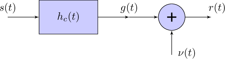
In practice, the channels have rather complicated responses (non-linear, time-varying, etc.). Fortunately, for many applications, a simple LTI model followed by AWGN provides a good match to the actual system under certain conditions. The combined effect of a LTI system denoted by its impulse response $h_{c} (t)$ with WGN $ν (t)$ added to the LTI system output leads to a received signal given by

r (t) = s (t) * h_{c} (t) + ν (t),

(4.1)

which is depicted in Figure 4.1 and is called here LTI Gaussian channel. This channel is called frequency-selective channel when its frequency response $H_{c} (f) = F {h_{c} (t)}$ varies with $f$ Another key aspect of the LTI Gaussian channel is that, because it is time-invariant, it is reasonable to eventually assume that it is known by both transmitter and receiver.

Figure 4.1: Block diagram of a LTI Gaussian channel.

Typically the channel model of Figure 4.1 can be classified according to the following features of the channel: a) equivalent to a lowpass or bandpass filter, b) ideal “brick-wall” magnitude flat-frequency response or frequency-selective (non-flat) filter and c) WGN at its output or not. The possible combinations of these three binary features require remedies that are widely used in digital communications, as illustrated in Table 4.1.

Table 4.1: Some channel features related to Eq. (4.1) and associated remedies.


Channel feature	Remedy

Flat (in frequency) over BW	Concentrate transmit signal spectrum within BW

Non-flat	Use equalizer or multicarrier modulation

AWGN	Use matched filter to maximize SNR

Bandpass	Use frequency upconversion to locate signal within BW

Assuming $h_{c} (t)$ is an ideal bandpass channel with center frequency $f_{c}$ , Table 4.1 indicates that the transmit signal should also have its spectrum approximately centered at $f_{c}$ by using frequency upconversion.

When $h_{c} (t)$ has a flat magnitude frequency response as, for example, the ideal lowpass in Figure E.1(a), it does not require equalization but most of the power of the transmit signal PSD should be confined within the channel bandwidth (BW). However, even with a flat magnitude, if $h_{c} (t)$ has a nonlinear phase, it may be still necessary to perform equalization. Note that Table 4.1 just indicates some of the possible remedies. For example, multicarrier transmission such as OFDM has been widely used to avoid the conventional equalizers in non-flat (or frequency-selective) channels. As will be discussed in Chapter 6, the idea in OFDM is to divide the non-flat channel in many small frequency bands (sometimes called “subchannels”) that can be considered approximately flat within their respective (small) bandwidth and, therefore, avoid complicated equalization (in fact, a 1-tap filter per subchannel is often used as equalizer in OFDM).

Whenever the channel has ideal frequency response (flat magnitude and linear phase) but is bandlimited, the channel $BW$ limits the maximum symbol rate $R_{sym}$ for achieving zero ISI, as will be discussed in this chapter. It should be noted that, even if $R_{sym}$ is bounded by a maximum value, if there was no noise ( $ν (t) = 0$ in Figure 4.1), the number $b$ of bits could be increased by using constellations with smaller spacing among symbols, and the rate $R = R_{sym} b$ could be made as large as desired.¹ Hence, generally speaking, $BW$ limits $R_{sym}$ , while the WGN power limits $b$ .

Assuming Eq. (4.1) specifies the channel of interest, it is pedagogical to study the effect of filtering and AWGN separately. Note that the optimal strategy may very well be to jointly combat the noise $ν (t)$ and the non-idealities of $h_{c} (t)$ .

By assuming that $h_{c} (t)$ is ideal, one can derive the matched filter as the optimal receiver for AWGN. Similarly, by discarding the influence of $ν (t)$ , one can design pulses to combat ISI due to the channel dispersion. Or in the case of a frequency-selective channel, one can assume an ideal equalizer can perfectly compensate the channel and use an AWGN model to study the system under this assumption of perfect equalization.

4.2.2 Flat-fading channel

A special case of the LTI Gaussian channel is the so-called flat-fading channel, depicted in Figure 4.2. This simpler channel is completely described by three parameters: $κ$ , $ϕ$ and $t_{0}$ , which are the channel gain, phase and delay, respectively. Assuming, for example, that $κ$ is a random variable with values that change over time allows to model effects that occur in wireless communications, for example.

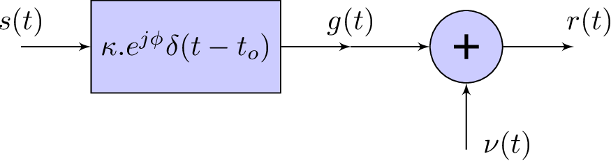
Figure 4.2: Flat-fading channel block diagram.

As depicted in Figure 4.2, the flat-fading impulse response is $h_{c} (t) = κ e^{jϕ} δ (t - t_{0})$ . Hence, the output $g (t)$ is related to the channel input $s (t)$ as

g (t) = κ e^{jϕ} s (t - t_{0})

(4.2)

and a simple scalar gain $1 ∕ (κ e^{jϕ})$ can be used as an equalizer for this channel.

The following sections discuss AWGN models, which are simpler than the flat-fading because the impulse response in Figure 4.1 can be modeled as $h_{c} (t) = δ (t)$ and, consequently, these channels have infinite bandwidth and are memoryless.

4.2.3 Discrete-time scalar AWGN

There are AWGN versions for continuous and discrete-time processing. The discrete-time AWGN channels can be further divided based on the fact that, at each channel use, a scalar (real or complex number) or a vector of dimension $D$ is transmitted. Figure 4.3 depicts some AWGN channels. An extra degree of freedom when modeling the discrete-time channels is whether the numbers represent symbols (at $R_{sym}$ ) or samples (at $F_{s}$ ).

Figure 4.3: Mind map with a possible taxonomy of AWGN channels.

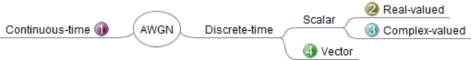
Complex numbers, such as the symbols in QAM modulation, can be modeled either as scalars or vectors of dimension $D = 2$ . In other words, when $D = 2$ , the fourth channel type in Figure 4.3 is equivalent to the third. For convenience, complex numbers will be treated as scalars in the sequel.

The scalar AWGN channel adds a noise sample $N$ to every transmitted scalar $x$ , which can represent a sample or a symbol. A distinction between having samples or symbols is that the assumed time interval between consecutive values of the corresponding sequences is $T_{s}$ or $T_{sym}$ , respectively.

As mentioned, the input $x$ is a real or complex number, such that the channel output is $R = x + N$ , where the random variable $N$ is i. i. d. and distributed according to a Gaussian PDF $N (0, σ^{2})$ with zero mean and variance $σ^{2}$ .

Example 4.1. Generating discrete-time real-valued scalar WGN. For example, a realization with 100 samples of a scalar discrete-time WGN can be easily obtained using Matlab/Octave with a command such as sigma2=0.5,N=100,noise=sqrt(sigma2)*randn(1,N), where $σ^{2} = 0.5$ W is the noise power. $□$

For a complex-valued $x$ , both real and imaginary parts of $N$ are often assumed i. i. d. and distributed according to $N (0, σ^{2})$ , such that the total power is $𝔼 [| N |^{2}] = 2 σ^{2}$ . More strictly, in this case, $N$ is a circularly-symmetric complex Gaussian² random variable distributed according to $C N (u, Σ)$ with zero mean $u = {[0, 0]}^{T}$ and covariance matrix $Σ = σ^{2} I$ , where $I$ is a $2 \times 2$ identity matrix.

Example 4.2. Generating discrete-time complex-valued WGN. Listing 4.1 is an example of code³ to generate discrete-time complex-valued WGN.

Listing 4.1: MatlabOctaveCodeSnippets/snip_digi_comm_gaussian_noise.m

1sigma2=0.5; %power per component (real and imaginary): 0.5 Watt 
2N=10000; %number of samples 
3noise=sqrt(sigma2)*randn(1,N)+1j*sqrt(sigma2)*randn(1,N); %complex 
4mean(abs(noise).^2) %estimate the noise power (approximately 1 Watt)

Note that after running Listing 4.1, the resulting power is approximately $𝔼 [| N |^{2}] = 2 σ^{2} = 1$ W, with 0.5 W per dimension. $□$

4.2.4 Discrete-time vector AWGN

As the name indicates, the vector AWGN channel adds a noise vector $ν$ to each transmitted vector $x$ (with symbols or samples as its elements), as depicted in Figure 4.4.

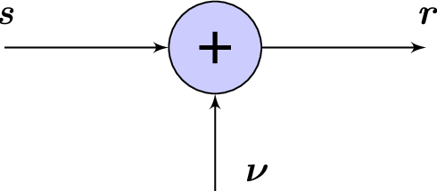
Figure 4.4: AWGN vector channel, where $s$ , $r$ and $ν$ are vectors of dimension $D$ .

The $D$ elements of vector $ν$ are i. i. d. random variables, each one distributed according to a Gaussian PDF with zero mean and variance $σ^{2}$ . Hence, the average power is $𝔼 {| ν |^{2}} = D σ^{2}$ .

As discussed in the context of signals (not vectors) in Application C.7, the output of the vector AWGN channel has power given by the sum of the powers of signal and the noise:

𝔼 {| r |^{2}} = 𝔼 {| s |^{2}} + 𝔼 {| ν |^{2}}

(4.3)

because $s$ and $ν$ are assumed to be orthogonal.

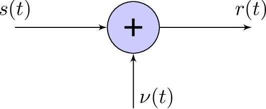
4.2.5 Continuous-time AWGN channel

The continuous-time AWGN channel can be represented as in Figure 4.5, where the noise $ν (t)$ is a realization of a WGN continuous-time WSS stochastic process.

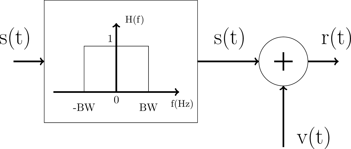
Figure 4.5: Continuous-time AWGN channel, which has the implicit assumption that $s (t)$ is both power and bandwidth-limited.

It is important to note that the continuous-time AWGN model assumes that the input signal $s (t)$ is both power and bandwidth-limited: its maximum power is $P_{s}$ and, in the baseband case, its support in frequency is from $- BW$ to BW assuming a bilateral representation. Hence, an alternative view to the AWGN in Figure 4.5 is to explicitly indicate the restricted bandwidth as in Figure 4.6, which depicts baseband and bandpass versions.

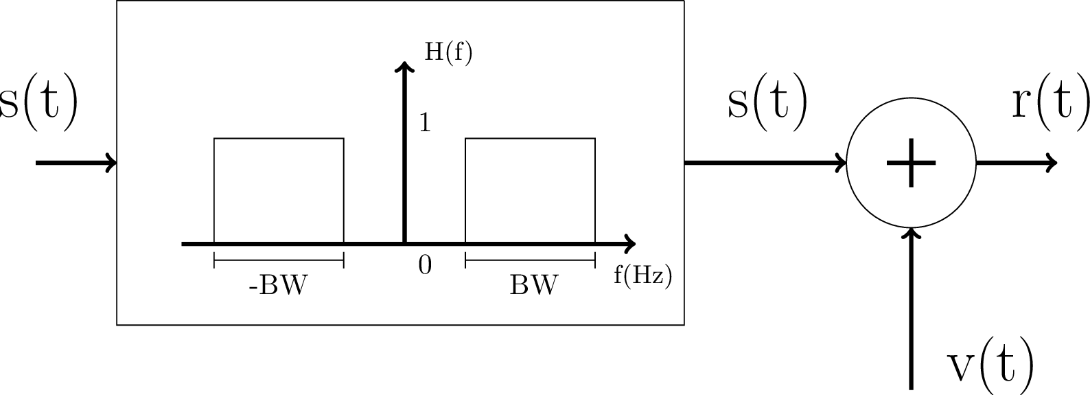
Figure 4.6: Lowpass (baseband) and bandpass continuous-time AWGN channels with the restriction in bandwidth made explicit. The input signal $s (t)$ is not altered because it is bandwidth-limited.

The continuous-time AWGN channels in Figure 4.6 should not be confused with the more general case of the LTI Gaussian channel of Figure 4.1. While, in Figure 4.1 any LTI system can be used, the systems in Figure 4.6 must be ideal and are depicted just in case one wants to make explicit that the input signal $s (t)$ is band-limited. In other words, two descriptions are equivalent:

f 1.: The AWGN corresponds to having an impulse response $h_{c} (t) = δ (t)$ in Figure 4.1. The channel has infinite bandwidth, but $s (t)$ has a limited bandwidth BW, or
f 2.: $h_{c} (t)$ is an ideal lowpass or bandpass filter, with a unitary gain (flat frequency response) and bandwidth BW, which does not alter the $s (t)$ .

In both cases, the essential fact is that the channel does not alter the band-limited $s (t)$ up to the point that it is added to $ν (t)$ .

The continuous-time AWGN model is very important for deriving theoretical results and, therefore, studying how to better implement practical systems. When using a computer to simulate a digital communication with DSP, the continuous-time AWGN is often mapped to a discrete-time AWGN model. This is discussed in Section F.7.3.

Note that, when simulating the AWGN channel using discrete-time processing, its bandwidth is not greater than $π$ rad or, equivalently, $F_{s} ∕ 2$ Hz, which is an inherent limitation of discrete-time processing. Besides, when simulating AWGN, there are no synchronization issues (after the channel, it is remains well-defined where each symbol starts and ends) and there is no intersymbol interference (ISI). This allows the transmission over AWGN to be treated as “one-shot”, i. e., modeling the channel effect over a single symbol without concerns on the influence of neighbor symbols, given that there is no ISI (detailed in Section 4.4). A zero-ISI transmission basically means that one symbol does not impacts the demodulation of other symbols. This way, the optimal receiver is a symbol-by-symbol detector that can make its decision based on a single use of the channel not on a sequence of uses (or sequence of symbols). On the other hand, when ISI exists, the decision may have to take in account a sequence of symbols and the optimum solution becomes more complicated, as discussed in Section 5.4.

4.2.6 LTI channel with non-white additive noise

In some situations of practical interest, the additive noise at the receiver may have a non-white PSD $S_{ν} (f)$ . For example, in DSL systems, the interference among distinct lines is often significant at a given receiver and it has a non-white PSD. In such cases, if its amplitudes are distributed according to a Gaussian, the noise is called additive Gaussian noise (AGN).

As discussed in Section F.10, parametric spectral estimation techniques can be used to estimate a filter $H (f)$ that, when excited by WGN, generates an output with a PSD that approximates $S_{ν} (f)$ . In some cases $H (f)$ can then be incorporated to the processing chain, creating a new system with a white noise that is equivalent to the original system with non-white noise, as represented in Figure 4.7.

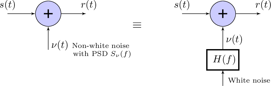
Figure 4.7: Two equivalent representations of non-white noise, where $H (f)$ is such that outputs a signal with PSD $S_{ν} (f)$ when its input is WGN.

It is possible to transform the system in Figure 4.7 into an equivalent AWGN system by moving the filter $H (f)$ to process the signal after the summation. Note that the Fourier transform $R (f) = F {r (t)}$ can be written as $R (f) = S (f) + W (f) H (f)$ , which is equivalent to $R (f) = (\frac{S (f)}{H (f)} + W (f)) H (f)$ , as indicated in Figure 4.8.

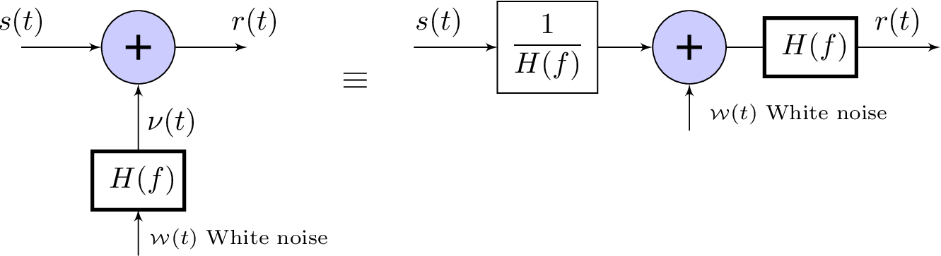
Figure 4.8: Signal processing trick to convert any AWN system into an equivalent AWGN.

The trick depicted in Figure 4.8 allows to transform any LTI system contaminated by non-white noise into an equivalent AWGN. This allows to use results available for AWGN such as matched filtering, discussed in the next section, and often simplifies the analysis of systems with non-white noise.

¹ It is also possible to increase $R$ by using higher transmit power but there is often a practical limit.

² See Appendix A.19.1 for a brief discussion about circular random variables. Figure 4.68 motivates the term circularly-symmetric, given that the 2-d pdf is “circular”.

³ When generating the imaginary component of noise, the value 1j was adopted instead of simply using j because j is often used as index and if previously defined with a value different than $\sqrt{- 1}$ , the simulation would go wrong. This is a potential problem when the code is large and it is always a good idea to use 1j or 1i to avoid this pitfall.