Applications

4.13 Applications

Application 4.1. The binary symmetric channel (BSC). In some applications it is convenient to represent signals as vectors and suppress waveforms. For example, in digital communications, the vector channel model assumes that $x$ and $y$ are the input and output vectors of a channel as indicated:

x → vector channel → y

and $x$ is a random vector with $M$ possible values.

The conditional probability $p(y | x)$ completely describes the channel and $y$ can have a continuous probability density function or a discrete probability mass function depending on $p(y | x)$ . If both cases are denoted as $p(y)$ , it is possible to write

p(y) = ∑_{i=0}^{M−1} p(y | x_{i})p(x_{i}).

Study the BSC channel and describe its distributions $p(y | x)$ and $p(y)$ when the input is uniformly distributed. Inspect the code MatlabOctaveBookExamples/ex_BSC_channel_capacity.m that explores the capacity of a BSC. $□$

Application 4.2. Alternatives for generating raised cosine filters: Matlab/Octave and GNU Radio. The raised cosine filter is often used in the context of digital communications. Because of that, most of the software to generate it has input parameters that are not used for designing regular filters. For example, the design of a raised cosine typically involves the concept of symbol rate $R_{sym}$ , which is of course never used in functions for general purpose filters such as fir1, firls, etc. Another fact is that most raised cosines are FIR filters, but it is possible to use IIR approximations too. Check the support to IIR filters in Matlab’s rcosine if interested. There are two popular FIR raised cosine filters: the “normal” and the square-root or RRC. The former is a Nyquist pulse that obeys Eq. (4.23) and is given by Eq. (4.29) while the latter is the discrete-time version of Eq. (4.33).

Listing 4.21 illustrates how to generate a normal FIR raised-cosine pulse using three alternatives and compares the first and third.

Listing 4.21: MatlabOctaveCodeSnippets/snip_digi_comm_raised_cosine_pulse.m

1Tsym = 1/8000; % Symbol period (s) 
2Fs = 24000; % Sampling frequency. Oversampling of 3 
3r = 0.5; % Roll-off factor 
4P = 31; % Pulse duration in samples, an odd integer 
5L = Tsym*Fs; %oversampling factor 
6groupDelay = (P-1)/(2*L); %group delay in samples 
7%1) Continuous-time version: 
8t = -groupDelay*Tsym:1/Fs:groupDelay*Tsym; %Sampling time 
9p = (sin(pi*t/Tsym)./(pi*t/Tsym)).*(cos(r*pi*t/Tsym)./ ... 
10    (1-(2*r*t/Tsym).^2)); 
11p(1:L:end)=0; %correct numerical errors: force zeros 
12p(groupDelay*L+1)=1; %recover the value due to 0/0 
13%2) Discrete-time version: (requires only L and r) 
14n = -groupDelay*L:groupDelay*L; %Sampling instants 
15p2 = (sin(pi*n/L)./(pi*n/L)).*(cos(r*pi*n/L) ./ ... 
16(1-(2*r*n/L).^2)); 
17p2(1:L:end)=0; %correct numerical errors: force zeros 
18p2(groupDelay*L+1)=1; %recover the value due to 0/0 
19%3) Use Matlab instead (not available on Octave): 
20%p3 = rcosine(1,L,'fir/normal',r,groupDelay); 
21%4) Use the companion function ak_rcosine (it mimics Matlab syntax) 
22p4 = ak_rcosine(1,L,'fir/normal',r,groupDelay); 
23%plot to compare two versions (they should be equal): 
24plot(p,'-+'),hold on,plot(p2,'r'),legend('Ver 1','Ver 2')

GNU Radio has the function gr.firdes.root_raised_cosine to design a RRC. Listing 4.22 provides an example.

Listing 4.22: Python_Language/raisedCosine.py

1import numpy 
2from gnuradio import gr 
3sps=3 #samples per symbol (or oversampling factor) 
4DCgain=20.0 #gain at DC in frequency domain 
5Rsym=500.0 #symbol rate (bauds) 
6Fs=Rsym*sps #sampling frequency (Hz) 
7rolloff=0.35 #rolloff factor (denoted as "alpha") 
8ntaps=13 #number of filter taps (must be an odd number) 
9rrcFilter=gr.firdes.root_raised_cosine(DCgain,Fs,Rsym,rolloff,ntaps) 
10numpy.savetxt('RRCfilter.txt',rrcFilter) #save as ASCII file

After successfully running Listing 4.22, the saved filter can be compared via Matlab/Octave using Listing 4.23.

Listing 4.23: MatlabOctaveCodeSnippets/snip_digi_comm_raised_cosine_GR.m

1p_gnuradio=load('RRCfilter.txt','-ascii'); %load file created by GR 
2L=3; %samples per symbol (or oversampling factor) 
3DCgain=20.0 %gain at DC in frequency domain 
4rolloff=0.35; %rolloff factor (denoted as "alpha") 
5ntaps=13; %number of filter taps (must be an odd number) 
6gDelay=(ntaps-1)/(2*L); %group delay (assuming linear phase FIR) 
7p=ak_rcosine(1,L,'fir/sqrt',rolloff,gDelay); %design square-root FIR 
8p=DCgain*(p/sum(p)); %gain at DC (sum(p) is the original DC gain) 
9plot(p_gnuradio,'o-'), hold on, plot(p,'rx-');%compare (should match)

Note that the gain at DC had to be imposed outside the function rcosine. $□$

Application 4.3. Zero ISI pulses. There is an infinite number of pulses that lead to zero ISI. To illustrate their formation law, Listing 4.24 exemplifies two cases, using random numbers.

Listing 4.24: MatlabOctaveFunctions/ak_generateZeroISIPulses.m

1function p=ak_generateZeroISIPulses(L,N,isLinearPhase,N0) 
2%function p=ak_generateZeroISIPulses(L,N,isLinearPhase,N0) 
3%Inputs: L - oversampling factor 
4%        N - determines the duration of p 
5%        isLinearPhase - set to 1 if p want linear phase 
6%        N0 - sample for obtaining the first symbol 
7if isLinearPhase 
8    if nargin > 3 
9        error('N0 cannot be used when isLinearPhase=1') 
10    end 
11else 
12    if N0 > N 
13        error('Sampling instant exceeds pulse duration') 
14    end 
15end 
16if isLinearPhase 
17    p=randn(1,L*ceil(N/2+1)); 
18    p(L:L:end)=0; 
19    p=[fliplr(p) 1 p]; 
20else 
21    p=randn(1,N*L+1); 
22    p(1:L:end)=0; 
23    p(1+(N0-1)*L) = 1; 
24end

For example, the commands randn(’seed’,0),p=ak_generateZeroISIPulses(2,2,1) led to p=[0 0.0751 0 1.1650 1.0000 1.1650 0 0.0751 0]. It is interesting to observe the spectra of pulses obtained with the command p=ak_generateZeroISIPulses(2,3,0,1) and p=ak_generateZeroISIPulses(2,3,0,2). In both cases, invoking ak_plotNyquistPulse(p,2) show $P_{s} (e^{j Ω})$ constant, as required for zero ISI. However, one should notice that ak_plotNyquistPulse uses the DFT to approximate the DTFT and this imposes some restrictions. For example, the pulse p=[2 1 3 0 3] leads to zero ISI, which can be confirmed with the commands:

Listing 4.25: MatlabOctaveCodeSnippets/snip_digi_comm_ak_calculateISI.m

1p=[2 1 3 0 3]; %shaping pulse 
2symbols=[3 -1 3 1]; %symbols used for all plots 
3L=2; %oversampling factor 
4N0=2; %sample to start obtaining the symbols 
5[isi,signalParcels] = ak_calculateISI(symbols, p, L, N0)

However, in this case, ak_plotNyquistPulse does not show the correct $P_{s} (e^{j Ω})$ . $□$

Application 4.4. Time evolution of a WGN orthogonal expansion. Eq. (4.8) was obtained for a given time instant. Assuming the correlative decoding scheme of Figure 2.26, the $n$ -th noise symbol ${\bar{N}}_{n}$ is obtained at $t = n T_{sym}$ . Each of the $D$ elements of ${\bar{N}}_{n}$ creates a random sequence $r_{i} [n]$ over time, which captures the evolution of the $i$ -th element of ${\bar{N}}_{n}$ . Depending on the duration of $φ_{i} (t)$ and $T_{sym}$ , the samples of $r_{i} [n]$ are correlated over $n$ or not. To study this correlation considering more than one instant, it is useful to recall the discussion about filtered AWGN in Section F.7.3 and also Example F.13. The first thing to note is that the correlation of $r_{i} [n]$ over time depends on the support of $φ(t)$ and the adopted time interval (e. g. $T_{sym}$ ) between expansions.

Here, the simplest case is adopted, in which $T_{sym} > φ_{i} (t)$ and the inner products $∫ ν(t) φ_{i} (t)dt$ are calculated over non-overlapping segments of duration $T_{sym}$ (e. g., $[n T_{sym},(n + 1) T_{sym}]$ ). In this case, there is no correlation over time as indicated by considering two time instants $k$ and $l$ :

\begin{array}{l} 𝔼[r_{i} [k] r_{i} [l]] & = 𝔼 [∫_{k T_{sym}}^{(k+1) T_{sym}} ν(t) φ_{i} (t)dt ∫_{l T_{sym}}^{(l+1) T_{sym}} ν(t) φ_{i} (t)dt] \\ = 𝔼 [∫_{k T_{sym}}^{(k+1) T_{sym}} ∫_{l T_{sym}}^{(l+1) T_{sym}} ν(t) φ_{i} (t)ν(s) φ_{i} (s)dtds] \\ = ∫_{k T_{sym}}^{(k+1) T_{sym}} ∫_{l T_{sym}}^{(l+1) T_{sym}} 𝔼 [ν(t)ν(s)] φ_{i} (t) φ_{i} (s)dtds \\ = ∫_{k T_{sym}}^{(k+1) T_{sym}} ∫_{l T_{sym}}^{(l+1) T_{sym}} R(t − s) φ_{i} (t) φ_{i} (s)dtds \\ = ∫_{k T_{sym}}^{(k+1) T_{sym}} ∫_{l T_{sym}}^{(l+1) T_{sym}} \frac{N_{0}}{2} δ(t − s) φ_{i} (t) φ_{i} (s)dtds \\ = \frac{N_{0}}{2} δ[k − l] ∫_{l T_{sym}}^{(l+1) T_{sym}} φ_{i}^{2} (t)dt = \frac{N_{0}}{2} δ[k − l]. & (4.97) \end{array}

In this case, $𝔼[r_{i} {[n]}^{2}] = 𝔼[N_{i}^{2}] = N_{0} ∕2$ W, as expected from Eq. (4.9), and there is no correlation over time for a given element of ${\bar{N}}_{n}$ .

In spite of the similarity of Eq. (4.97) and Eq. (4.8), they are distinct in the sense that Eq. (4.8) indicates the elements of an orthogonal expansion of WGN are always uncorrelated among them, while Eq. (4.97) takes time into account and depends on $T_{sym}$ and the durations of ${φ_{i} (t)}$ . The next paragraphs further discusses this issue.

First, consider the example of Listing 2.22 where correlation and convolution are made equivalent. This equivalence suggests interpreting the correlative decoding scheme in Figure 2.26 as simultaneously filtering with a set of $N$ orthonormal functions ${φ_{i}},i = 1,…,N$ and periodically sampling the output with interval $T_{sym}$ . Note that ${φ_{k}}$ plays the role of a set of impulse responses composing a filter bank with $N$ filters. This interpretation is used in the sequel.

As mentioned, if the interval $T_{sym}$ is longer than the impulse responses, the filters do not correlate the noise at their inputs. To illustrate a case where this is not the case, a Matlab/Octave code was created using the same $D = 2$ basis functions of Figure 2.32. The received signal $r[n] = ν[n]$ is simply WGN, stored in array noise and representing a discrete-time version of $ν(t)$ . Some relevant lines of this code are shown in Listing 4.26.

Listing 4.26: MatlabBookFigures/figs_digi_comm_awgn_decomposition

18%... (preceded by some code) 
19noisePower = 20; %AWGN power in Watts 
20noise=sqrt(noisePower)*randn(S*L,1); %generate AWGN noise 
21for n=1:D %loop over all basis functions 
22    innerProductViaConv(n,:)=transpose(conv(noise,fliplr(A(:,n)'))); 
23    rxSymbols(n,:)=innerProductViaConv(n,L:L:end); %decimate 
24end 
25[R1,lags]=xcorr(innerProductViaConv(1,:),30); %without decimation 
26[R2,lags]=xcorr(innerProductViaConv(2,:),30); %without decimation 
27[R1d,lags]=xcorr(rxSymbols(1,:),30); %decimation 16:1 (D=16) 
28[R2d,lags]=xcorr(rxSymbols(2,:),30); %decimation 16:1 (D=16) 
29P=floor(S/L); %num. of vectors for estimating covariances (P <= S/D) 
30C=cov(transpose(innerProductViaConv(:,L:P))) %covariance 
31Cd=cov(transpose(rxSymbols(:,1:P-L+1))) %use sequences with P values 
32%... (followed by some code)

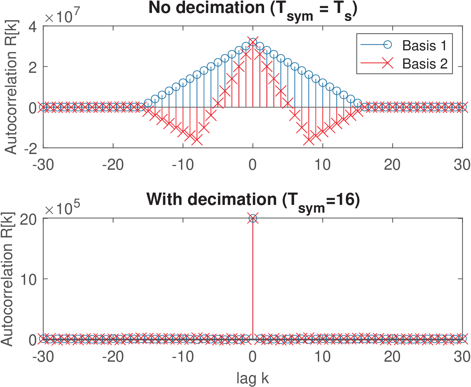
The two main signals in Listing 4.26 are innerProductViaConv and rxSymbols. The array innerProductViaConv stores the samples obtained at the output of the two correlators, at a rate corresponding to $F_{s}$ . In contrast, rxSymbols is a decimated version of innerProductViaConv, by a factor $L = 16$ to 1. Given the assumed $T_{sym} = 16$ , this decimation corresponds to having rxSymbols at the symbol rate $R_{sym}$ . Figure 4.67 shows the autocorrelations for the output signals considering these two options and the $D = 2$ basis functions.

As depicted in Figure 4.67, if the symbols are extracted with a long enough time interval ( $T_{sym}$ , in this example), Eq. (4.97) holds and the noise sequences $r_{i} [n]$ do not present strong correlation over time as shown in the bottom plot of Figure 4.67 (which plots R1d and R2d in Listing 4.26). In contrast, the top plot (plots R1 and R2 in Listing 4.26) shows the influence of the filtering operation that correlates the noise.

Figure 4.67: Comparison of autocorrelations for the signals at the outputs of the $D = 2$ correlators at $F_{s}$ (top) and $R_{sym}$ (bottom) rates.

Agreeing with Eq. (4.8), The correlation matrices generated by Listing 4.26, corresponding to innerProductViaConv and rxSymbols, were:

     C =[18.5811   -0.0050   and   Cd =[19.9123   -0.3484
        -0.0050   20.2618]              -0.3484   20.0750]

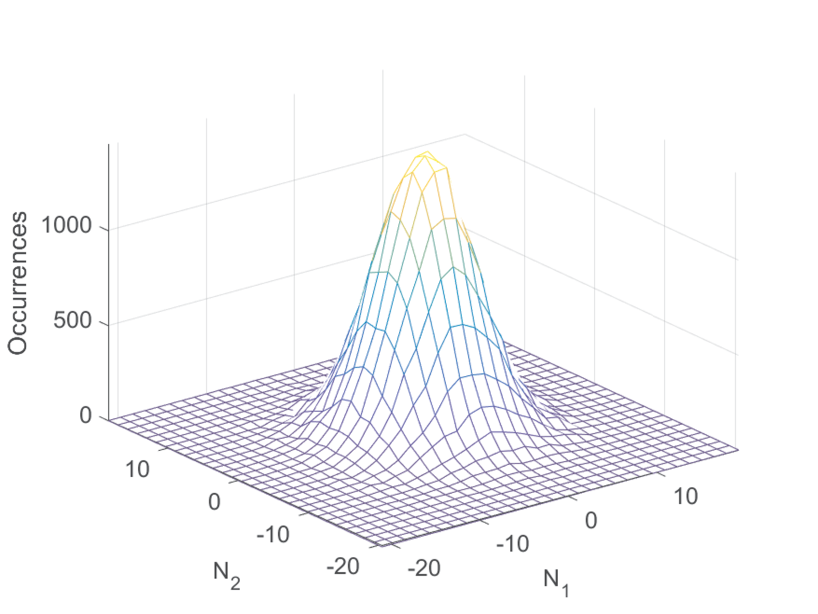
Hence, another view of the correlator action can be depicted as in Figure 4.68, which shows that the two-dimensional histogram of $[N_{1}; N_{2}]$ (columns of rxSymbols) resembles a Gaussian.

Figure 4.68: Histogram of vectors $[N_{1}; N_{2}]$ from rxSymbols in Listing 4.26.

The diagonal elements for both matrices C and Cd are approximately the specified noise power of 20 W. But note that the out-of-diagonal elements of Cd (with decimation) are almost $0.3484∕0.005 ≈ 70$ times the one of C (without decimation). According to Eq. (4.8), both should be $𝔼[N_{1} N_{2}] = 0$ . In practice, results such as $𝔼 [ν(t)ν(s)] = \frac{N_{0}}{2} δ(t − s)$ used in Eq. (4.8), are impacted by the finite number of samples to estimate statistics. The example used only P=6250 vectors and better estimates can be achieved by increasing this number.

Figure 4.69 provides a frequency-domain interpretation of Figure 4.67 using the first basis function.

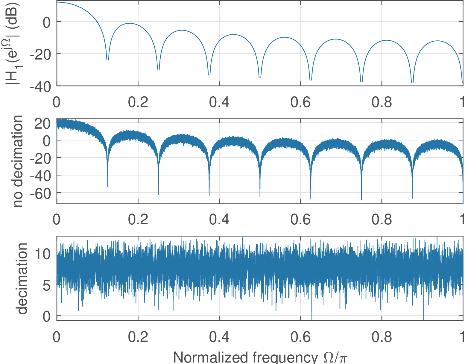
Figure 4.69: Frequency domain interpretation of Figure 4.67 using the first basis function: the filter gain (top), PSDs of output signal at rate $F_{s}$ and $R_{sym}$ (bottom).

The PSD of rxSymbols(1,:) (bottom plot in Figure 4.69) is approximately white, while the PSD of innerProductViaConv(1,:) is imposed by the corresponding basis function. $□$

Application 4.5. Introduction to GSM using GSMsim. This application briefly discusses the GSM physical layer (PHY), which simultaneously uses frequency (FDMA) and time-division multiplexing (TDMA) in its multiple-access architecture [Yac02]. In frequency, the radio channels are separated by 200 kHz and each channel is split in time domain to enable eight time slots. To obtain full-duplex transmission, GSM adopts frequency division duplexing (FDD) with up and downlink typically separated by 45 MHz and uplink using lower frequencies than downlink. But the FDD frequency separation is 80 MHz in GSM-1900, for example, which adopts bands of 60 MHz in contrast to the standard (or primary) bands of 25 MHz called P-GSM-900.

In fact, the original GSM-900 system, with the P-GSM-900 frequency bands around 900 MHz evolved in several variants, such as the ones operating at 1.8 and 1.9 GHz and called GSM-1800 and GSM-1900, respectively.²⁵ Hereafter, the GSM-900 system is assumed.

In a given channel, GSM transmits a total of 1,625 symbols within an interval of 6 ms. Hence, the symbol period is $T_{sym} = 6∕1625 ≈ 3.6923$ $μ$ s and the symbol rate $R_{sym} = 1∕ T_{sym} ≈ 270.833$ kbauds. This corresponds to $270.833$ kbps when GSM uses Gaussian Minimum-Shift Keying (GMSK) binary modulation. GSM systems adopt GMSK for voice calls and also for packet-oriented mobile data services using the General Packet Radio Service (GPRS). Note that GMSK uses a constellation with $M = 4$ symbols but the adopted differential encoding leads to only $b = 1$ instead of $b = 2$ bits per symbol: a bit 0 is encoded by a clockwise change in phase (for example, from phase $Θ$ to $Θ − π∕2$ rad), while a bit 1 corresponds to a counter clockwise change (from $Θ$ to $Θ + π∕2$ rad).

In GPRS, the net bit rate varies according to the adopted channel coding scheme, which can use code rates from 1/2 to 1. But the GPRS modulation is always GMSK with $b = 1$ . To support higher data rates, EDGE (Enhanced Data rates for GSM Evolution) uses not only GMSK but also 8-PSK ( $b = 3$ ). The following discussion will assume GMSK.

GMSK is a constant envelope modulation that, for transmitting the mentioned $270.833$ kbps, requires a bandwidth of approximately 270.833 kHz. Given that GSM radio channels are separated by 200 kHz, they overlap in frequency. This overlap is not a problem because, guided by the so-called frequency reuse adopted in cell planning, the transceiver of a given cell does not use channels in adjacent carrier frequencies. Hence, GSM can pack 125 channels in one direction (up or downlink) in $125 × 200 kHz = 25$ MHz but they will not be simultaneously used in a given cell. Typically, a single cell uses from one to 16 pairs of frequencies, for up and downlink.

The radio channel is time-multiplexed into eight time slots (TS) and are called TS0 to TS7. Together, these eight TS compose a frame of 1,250 symbol periods. The frames are organized in multiframes of 26, 51 or 102 frames. For example, the control channel multiframe is composed of 51 frames and has a duration of 235.38 ms, while the traffic channel multiframe is composed of 26 frames and has a duration of 120 ms. Every cell has to transmit, at least in one of its frequency and at TS0, the control channel multiframe. In downlink it provides information for frequency correction and synchronization, while in uplink it provides the random access channel (RACH) that is used by the mobile to establish the initial conversation with the base station.

Each TS has a duration of $1,250∕8 = 156.25$ symbol periods that corresponds to $156.25 × T_{sym} ≈ 576.9$ $μ$ s. These 156.25 symbols compose a burst.

In a GSM burst, 148 symbol intervals correspond to actual data or, equivalently to 148 bits. The remaining 8.25 symbol intervals are guard intervals to prevent bursts from overlapping and interfering with transmissions in other time slots. Hence, a maximum of 148 bits can be transmitted in each TS (576.9 $μ$ s).

There are five main types of bursts in GSM: normal (NB), frequency correction (FCB or FB), synchronization (SB), access (AB) and dummy burst. These bursts are used by different logical channels to perform specific tasks. GSM allows only certain combinations of logical channels and bursts.

The FB is used for frequency synchronization of the mobile station. It has the same guard time as a normal burst (8.25 symbols). The broadcast of the FB usually occurs on the logical channel called frequency correction channel or FCCH. FB has 3 tailing bits in each side and 142 bits equal to zero, which implies that the constellation symbols are picked by moving counterclockwise in the constellation, with a difference of $− 90$ degrees between consecutive symbols. The corresponding signal is a tone (sinusoid) with a nominal frequency of 67.7 kHz, corresponding to 1/4 of the symbol rate.

The so-called “Combination V” C0T0 beacon is the following control channel multiframe, which is permanently sent by the base station at channel zero (C0) and time slot 0 (T0):

     FSBBBBCCCCFSCCCCCCCCFSCCCCCCCCFSCCCCCCCCFSCCCCCCCCI
     F: FCCH (Frequency Correction Channel)
     S: SCH  (Synchronization Channel)
     B: BCCH (Broadcast Control Channel)
     C: CCCH (Control Channel) obs: 3 first quartets are
             CCCH while other 4 quartets are SACCH
     I: Idle (Mobile can decode information from other base stations)

The handsets monitor C0T0 and can identify when they are being called and when they can call the base station.

There is a FCCH burst every 10 bursts on the TS0. The FCCH is always followed by a SCH burst. Note the C0T0, as others logical channels, occurs in one specific time slot, so one needs to wait 7 physical time slots to get the SCH that follows a FCCH. Recall that each TS corresponds to 156.25 symbols (or bits) and, therefore, seven time slots correspond to $156.25 × 7 = 1093.75$ symbols.

The information from the SCH allows us to calculate the Frame Number (FN). For each burst the FN is incremented by 1 until it reaches $8 × 26 × 51 × 2048$ . It then starts at 1 again. If we modulo 51 the FN we know exactly if the current burst is at the beginning of a 51-multiframe or somewhere else. The SCH also tells us about the Base Station Color Code (BCC) and the Network Color Code (NCC).

The next paragraphs discuss GSMsim, a simulator that is useful to practice the discussed concepts. A more advanced simulator can be found at [ url7gmp], which implements the GSM PHY code in Matlab with interface to L2/L3 of the OsmocomBB project. The GSMsim is used in the sequel due to its simplicity.

GSMsim²⁶ is a GSM toolbox for Matlab/Octave. The original and a slightly modified versions can be found at the companion software, directory Applications/GSMsim. A modified version of the code is in folder ak_GSMsim, and this version will be assumed here. The manual GSMsim_manual.pdf provides a comprehensive description of the toolbox.

To use the code in Matlab/Octave, first go to the folder Applications/GSMsim/ak_GSMsim/config and execute the script GSMsim_config.m. It will set a variable called GSMtop that contains the full path of GSMsim’s main folder and include its five subdirectories in Matlab/Octave’s path. After that, one can run the main scripts that are in folder Applications/GSMsim/ak_GSMsim/examples with commands such as:

1ak_GSMsim_demo 
2ak_GSMsim_demo_2_withChannelCoding

The code below shows how to generate the IQ samples and plots the I component.

1gsm_set 
2BURST=-1+(2*(rand(1,148)>0.5)); 
3[I,Q] = gmsk_mod(BURST,Tb,OSR,BT); 
4plot(I);

The code below illustrates how to generate the complex envelope of a GSM signal and obtain its PSD.

1gsm_set; %set some variables 
2numOfBurts = 500; %number of bursts 
3numOfSamples = 150*OSR;%number of burst samples 
4gsmComplexEnvelope = zeros(1,numOfBurts*numOfSamples); 
5startSample = 1; 
6endSample = startSample + numOfSamples - 1; 
7for n=1:numOfBurts; 
8    tx_data = data_gen(INIT_L); %randomly generate a burst 
9    %modulate a burst 
10    [burst, I, Q] = gsm_mod(Tb,OSR,BT,tx_data,TRAINING); 
11    gsmComplexEnvelope(startSample:endSample) = I + j*Q; 
12    %update for next iteration: 
13    startSample = endSample + 1; 
14    endSample = startSample + numOfSamples - 1; 
15end 
16Fs = OSR * 270833; %sampling frequency in Hz 
17N=1024; 
18pwelch(gsmComplexEnvelope,N,[],N,Fs)

Listing 4.27 illustrates how to perform a simulation using GSMsim. In this case, 100 bursts were generated. The channel was AWGN with approximately 14 dB of SNR.

Listing 4.27: ./Applications/GSMsim/ak_GSMsim/examples/ak_GSMsim_demo.m

1numOfBurts =500; %number of bursts 
2Lh=2; %channel dispersion: length of the channel impulse 
3      %response minus one. 
4shouldAddNoise = 1; %add AWGN noise if 1 
5gsm_set; %set some important variables 
6%pre-compute tables used by Viterbi: 
7[SYMBOLS,PREVIOUS,NEXT,START,STOPS] = viterbi_init(Lh); 
8B_ERRS=0; %reset counter for number of bit errors 
9for n=1:numOfBurts 
10    tx_data = data_gen(INIT_L); %randomly generate a burst 
11    %modulate a burst 
12    [burst, I, Q] = gsm_mod(Tb,OSR,BT,tx_data,TRAINING); 
13    %pass signal over the channel 
14    if shouldAddNoise == 1 
15        [r,snrdB]=channel_simulator(I,Q,OSR); 
16        if n==1 %show SNR only for the first burst 
17            disp(['SNR = ' num2str(snrdB) ' dB']); 
18        end 
19    else 
20        r = I + 1j*Q; %no channel: noise and ISI free 
21    end 
22    %matched filtering: 
23    [Y, Rhh] = ak_mafi(r,Lh,T_SEQ,OSR); 
24    %decoding using Viterbi: 
25    rx_burst = viterbi_detector(SYMBOLS,NEXT,PREVIOUS,... 
26        START,STOPS,Y,Rhh); 
27    rx_data=DeMUX(rx_burst); %demultiplexing 
28    B_ERRS=B_ERRS+sum(xor(tx_data,rx_data)); %count errors 
29end 
30BER=(B_ERRS*100)/(numOfBurts*148); %calculate BER 
31fprintf(1,'There were %d Bit-Errors\n',B_ERRS); 
32fprintf(1,['This equals %2.1f Percent of the checked ' ... 
33    'bits.\n'],BER);

The source code can be easily modified for changing parameters of interest. $□$

Application 4.6. Analyzing GSM data. This application discusses an analysis of a file²⁷ containing a GSM signal and used at the “GSMSP Challenge”. To obtain this file, the DDC of the USRP was setup to perform anti-aliasing (analog) filtering, down-converting the signal at the original radio frequency (RF) of 953.6 MHz to baseband and eliminating the undesirable image spectra. The baseband complex-valued signal was sampled at 64 MHz and decimated by a factor of 128. Therefore, the file stores a complex signal sampled at $f_{s} = 500$ kHz and has 80,000 samples, which corresponds to a duration of 160 ms.

The analysis method that will be discussed was used by the winner of the GMSP Challenge. Before running this code, one needs to execute GSMsim_config.m as explained in Application 4.5. The code was commented and slightly modified, and can be found at directory Applications/GSM_PHY_Analysis. The following commands are called from the main script ak_runAllSteps.m:

1clear all, gsm_setGlobalVariables, ak_step1a, ... 
2    ak_step1b, ak_step1c, ak_step2a, ak_step2b, ak_step3

and allow to partially decode the signal as will be discussed here.

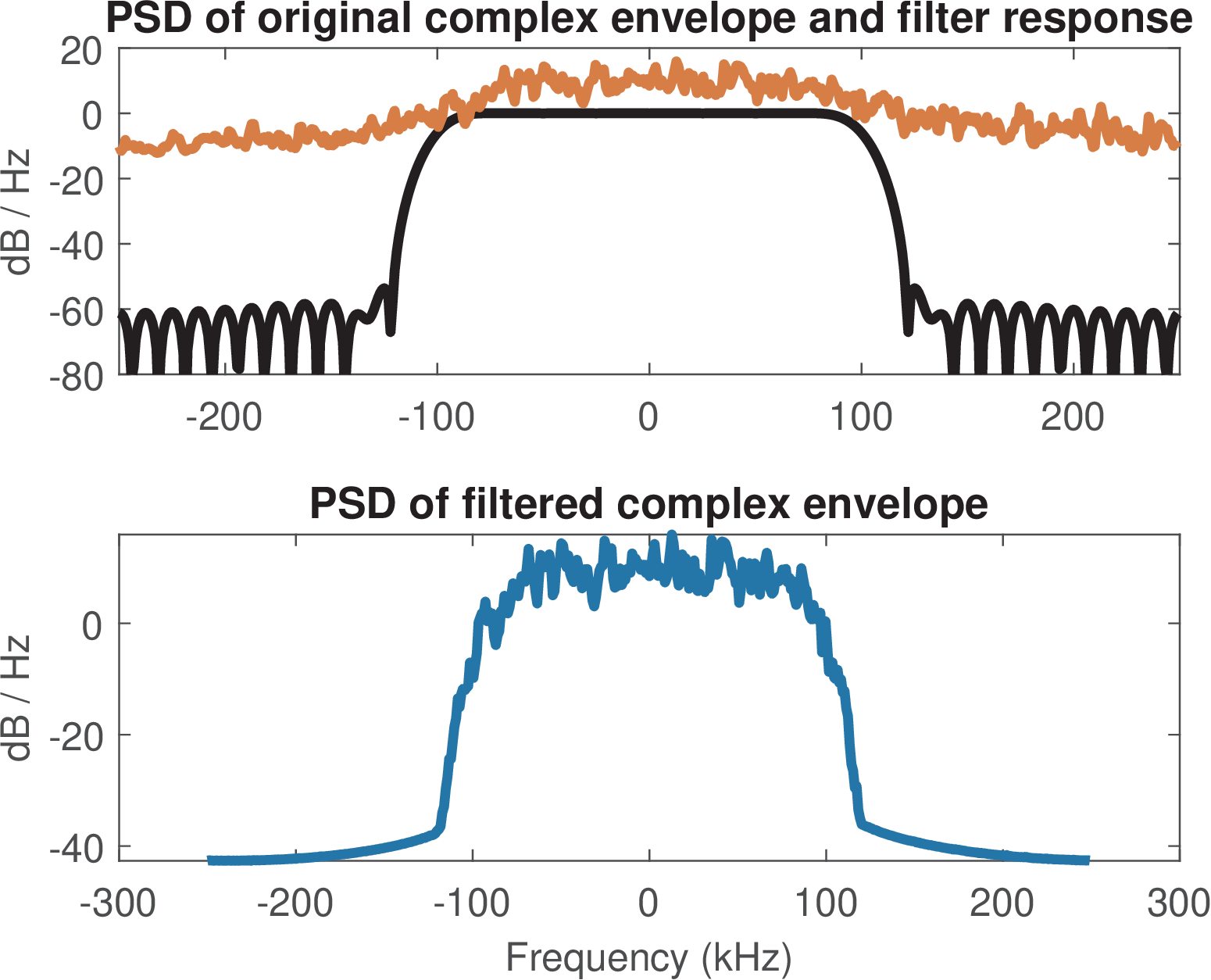
Using ak_step1a, the original signal is lowpass filtered for improved performance using a FIR filter of order 60. This filter was designed using the windowing method with a Hamming window through the Matlab command h = fir1(60,0.4), where the desired cutoff frequency $f_{c} = 100$ kHz (to account for a spectrum of interest in the range $− 100$ to $100$ Hz of the complex-valued signal) is normalized to $f_{c} ∕(f_{s} ∕2) = 0.4$ as required by Matlab/Octave. Figure 4.70 illustrates the PSDs and the filter’s frequency response $H(f)$ . The graph depicts the magnitude $|H(f)|$ in dB, which shows that the filter has a gain of 0 dB at 0 Hz.

Figure 4.70: PSDs of original and filtered signals. Note that the PSDs do not present Hermitian symmetry because the original and filtered signals are complex-valued.

It is convenient to process the signal sampled at multiples of the symbol rate $R_{sym} = 270,833$ bauds. In Matlab/Octave, changing $f_{s}$ to a new value $F_{s} = (P∕Q) f_{s}$ , with $P,Q ∈ ℕ$ can be conveniently done with the function resample. The resample adopts, by default, a 10-th order FIR filter to perform interpolation and to combat aliasing before decimation.

A first task is to estimate the frequency correction by finding FB, the corresponding FCCH burst. The FB is used for compensating mismatches in the radio front end, such as in the local oscillator. A receiver such as the USRP typically does not achieve the exact carrier frequency used by the transmitter in the down-conversion process, and imposes an offset frequency (or error) to the generated baseband signal.

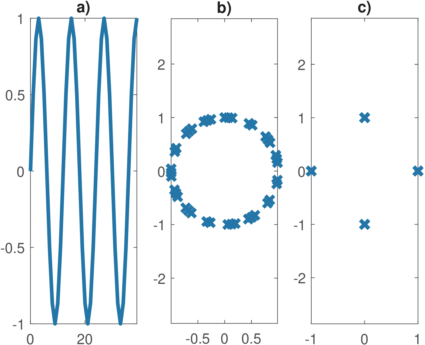
Figure 4.71: Generated by Listing 4.28: a) is the FB burst, b) is the received constellation when there is a frequency offset of 0.1 rad and c) is the corrected constellation.

Listing 4.28 illustrates how a frequency offset impacts the received symbols. The code was used to obtain Figure 4.71. In this code, an offset of 0.1 rad was imposed, estimated and corrected. This is the base of the procedure that will be used to correct the offset for the digitized GSM signal.

Listing 4.28: ../Applications/GSM_PHY_Analysis/ex_gsm_freq_correction

1const=[1 1j -1 -1j]*exp(1j*pi/2); %QPSK constellation 
2wc=2*pi/3; %carrier frequency 
3N=40; %number of symbols 
4n=0:N-1; %discrete-time index 
5%picking symbols counterclockwise to generate FB 
6s=const( rem(n,4) + 1 ); 
7txcarrier=exp(-1j*wc*n); %carrier at transmitter 
8x=s.*txcarrier; %modulated signal, oversampling = 1 
9%simulate a demodulation with frequency error 
10dw = 0.1 %error (frequency offset) in rad 
11rxcarrier=exp(1j*(wc+dw)*n); %carrier at receiver 
12sq=x.*rxcarrier; %demodulated signal 
13%trick to find the angle differences between samples: 
14angleDiff=angle(sq(1:N-1).*conj(sq(2:N))); 
15%estimate frequency offset: 
16dw_estimated = -pi/2 - mean(angleDiff) %in rad 
17%compensate freq offset: 
18sq_corrected=sq .* exp(-1j*dw_estimated*n);

To estimate the frequency offset using a FB, it is necessary to find the FB. This procedure can be computationally demanding and working at the baud rate alleviates this cost. For the example under discussion, the resample function was used with $P = 13$ and $Q = 24$ , to convert the original signal sampled at 500 kHz to a new signal x with $F_{s} = (13∕24)500,000 = 270,833$ Hz. This is below the minimum sampling frequency stated by the sampling theorem (there is loss of information) but it is enough for the frequency offset estimation. The complex samples of the resampled signal correspond to symbols, potentially shifted in time and frequency.

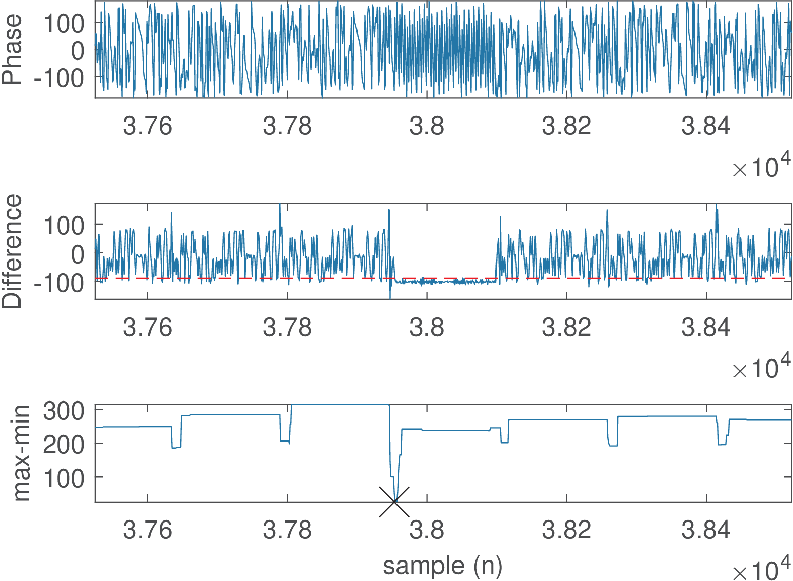
Figure 4.72: Location of a burst for frequency correction. All graphs are in degrees, not rad. The top plot a) shows the phase $p[n]$ of received symbols, b) is the difference $p[n] − p[n − 1]$ with a line indicating a difference of $− 90$ and c) indicates the estimated start sample.

The task is to find the (approximate) beginning of the FHCC payload. Note that 148 symbols correspond to 148 samples if the oversampling is one, but only 142 symbols will be used because 6 out of the 148 are tailing bits. Ideally, all the angle differences between consecutive symbols are $− 90$ degrees. In this ideal case, both the minimum min and maximum max values of this difference value over the search interval is $− 90$ and max-min=0. Therefore, the adopted procedure is to use a sliding window with length of 146 symbols to search the sample where the difference between the maximum and minimum values of angleDiff is minimum. When random bits are transmitted, this difference will be as large as $2π$ rad and an arbitrary threshold of 1 rad (in the range $[0,2π]$ ) was used to detect FBs. If the minimum dynamic range max-min is less than 1 rad, it is assumed a FB was found. Figure 4.72 illustrates the result of this procedure, which identified a FCCH start at sample number 12962.

One method for calculating the phase difference $𝜃[n] − 𝜃[n + 1]$ between two consecutive samples is

1angleDiff=angle(x(1:L-1).*conj(x(2:L)));

where x is the resampled signal and L its length.

Extracting the phase is important in GMSK. The following code investigates alternatives.

1r=exp(j*([1 2 3 4 5])); %example of phase (adding 1 rad) 
2L = length(r); %number of samples of interest 
3%first method to obtain the phase difference: 
4da = angle(r(1:L-1) .* conj(r(2:L))); %angles difference 
5%second method, which does not unwrap the phase 
6da2 = - filter([1 -1],1,angle(r)); %H(z)=1-z^(-1) 
7da2(1)=[]; %take out the filter transient 
8%third method unwraps phase. It's equivalent to the first 
9da3 = - filter([1 -1],1,unwrap(angle(r))); %unwrap before 
10da3(1)=[]; %take out the filter transient

Note that it is important to properly deal with phase wrapping in this situation.

After having the phase difference, the cumulative sum of these differences gives back the phase. In Matlab/Octave, this can be accomplished with

1angleSum=cumsum(angleDiff);

Figure 4.73: Angle differences for the detected frequency correction burst, where the indicated average is the frequency offset of 0.2017 radians.

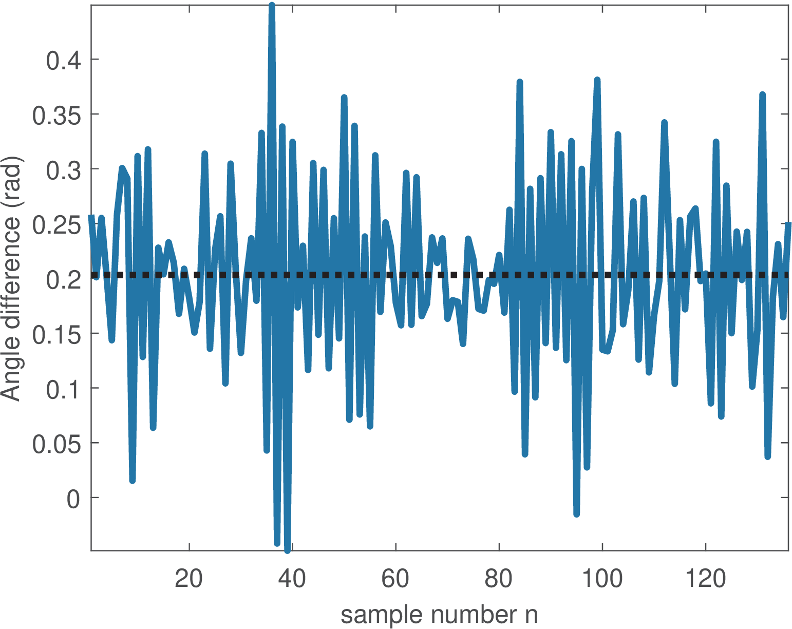
Figure 4.73 illustrates the estimated offset of $Δ Ω = 0.2017$ rad for the signal under analysis. It is a zoom of the FB at Figure 4.72, plot b). The offset corresponds to $Δ f = Δ Ω × F_{s} ∕(2π) = 0.2017 × 270,833∕(2π) = 8,695.6$ Hz. A new signal y = x $e^{−j Δ Ω}$ is obtained by translating the spectrum of x to correct the estimated offset.

Note that, if there is oversampling (OSR>1), then the expected phase change will not be 90 degrees but 90/OSR. In Matlab/Octave, this corresponds to

1angular_freq_offset = -(pi/2/OSR) - mean(angleDiff) %rad

After identifying the FB, the next task is to find the SCH burst that follows the FCCH. Because the oversampling factor is 4, the number of samples from the beginning of the FCCH to the start of the SCH is $156.25 × 8 × 4 = 5000$ samples.

Listing 4.29: Applications/GSM_PHY_Analysis/find_sch.m

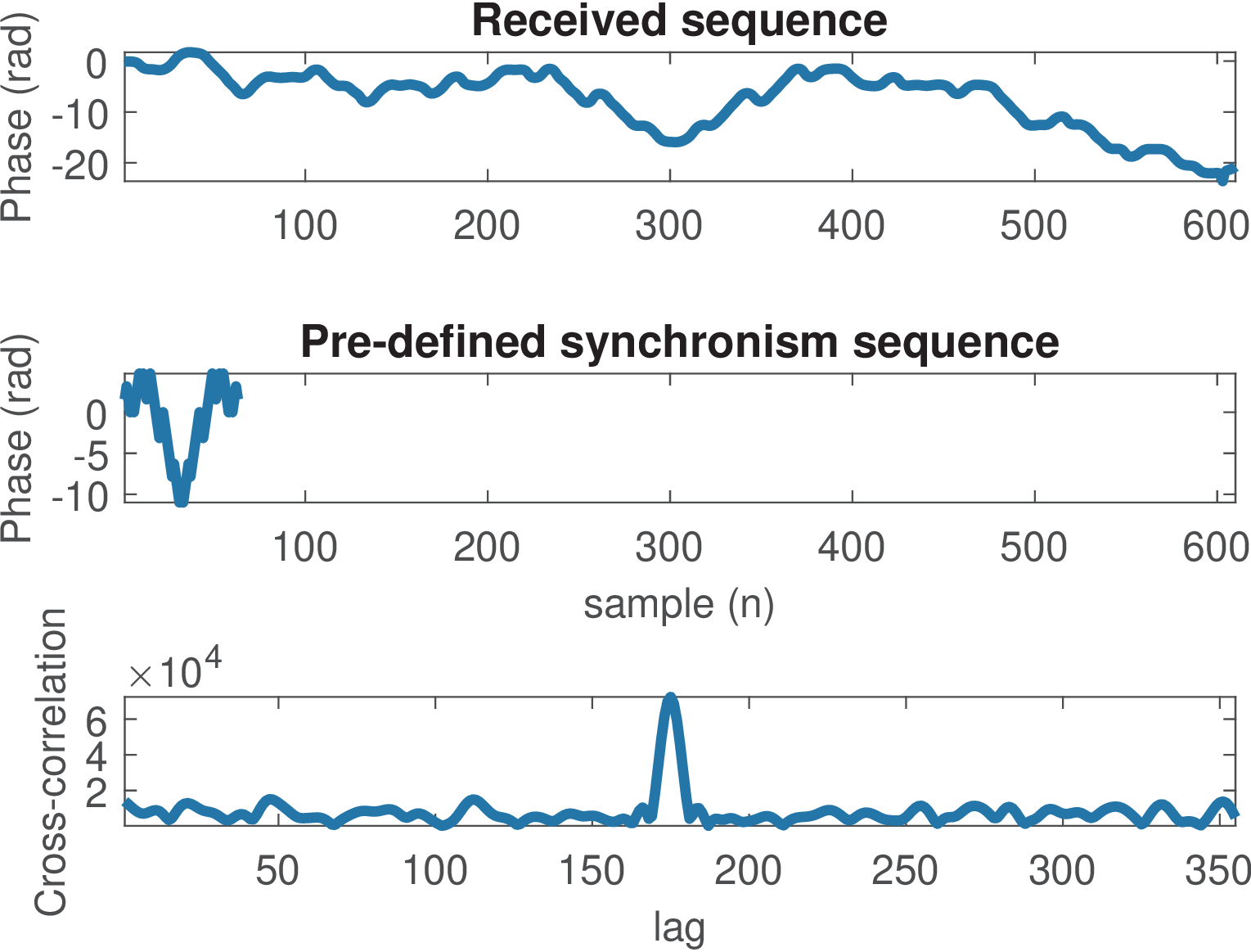
1function [sch_startViaSCH, crossCorrelation, lags]=find_sch(r, start) 
2%function [sch_startViaSCH, crossCorrelation, lags]=find_sch(r,start) 
3%Find SCH burst beginning. Inputs: 
4% r -> GSM signal 
5% start -> estimated sample to start the SCH 
6%Recall that the SCH burst has 
7%3 tail bits | 39 coded bits | 64 bits training seq. | 39 coded ... 
8%bits | 3 tail bits | 8.25 guard period bits 
9%Assumes signal is oversampled by 4 times the symbol rate. 
10global syncSymbols 
11if ~exist('syncSymbols','var') 
12    error(['Globals not defined. Run the script' ... 
13        ' gsm_setGlobalVariables.m']) 
14end 
15OSR = 4; %oversampling ratio 
16%limit the search range to 610 samples (152.5 symbols) 
17if start + 610 > length(r) 
18    sch_startViaSCH=-1; 
19    crossCorrelation=-1; 
20    lags=-1; 
21    warning('find_sch: not enough samples!') 
22    return 
23end 
24a = r(start:start+610); 
25numSyncSamples = OSR*length(syncSymbols); 
26%number of samples of a that can be used in correlation: 
27N = length(a)-numSyncSamples; 
28crossCorrelation = zeros(1,N); %pre-allocate space 
29for lag = 1:N 
30    %extract segment of vector a with size equal to 
31    %the size of syncSymbols and also same symbol rate 
32    segment = a(lag:OSR:lag+numSyncSamples-OSR); 
33    %crosscorrelation at lag is an inner product 
34    %(syncSymbols is a row vector and segment a column): 
35    crossCorrelation(lag)= syncSymbols * conj(segment); 
36end 
37%find the crosscorrelation peak: 
38[maxCorrelation, location] = max(abs(crossCorrelation)); 
39%Make a correction to point to the beginning of the SCH 
40%Recall that the SCH burst has 
41%3 tail bits | 39 coded bits | 64 bits training seq. | 39 coded ... 
42%bits | 3 tail bits | 8.25 guard period bits 
43%so, there are 42 = 39 + 3 bits before the training sequence 
44%Because OSR=4, 42 symbols correspond to 168 samples 
45%sch_startViaSCH = start-1 + location - OSR*42; 
46%AK: this -7 is empirical 
47sch_startViaSCH = start-1 + location - OSR*42 - 7; 
48lags = 1:N; %define array lags that is part of the function output

Listing 4.30: MatlabOctaveBookExamples/ex_crossCorrelationDiffRates.m

1%create two sequences: s1 at baud rate and s2 oversampled 
2OSR=4; %oversampling factor 
3N1=3; %number of samples of sequence s1 
4N2=2*OSR*N1; %number of samples of sequence s2 
5s1 = (1:N1)*(1+j); %at baud rate (OSR=1) 
6s2 = (1:N2)*(1-0.5*j); %at OSR times baud rate (OSR>1) 
7%First method - not using the xcorr function 
8%number of samples of s2 that can be used in correlation: 
9N = N2-OSR*N1; 
10%make s2 a column vector. Prepare for inner product 
11s2=transpose(s2); 
12crossCorrelation = zeros(1,N); %pre-allocate space 
13for lag = 1:N 
14    %extract segment of s2 with size and rate equal to s1 
15    segment = s2(lag:OSR:lag+(N1-1)*OSR); 
16    crossCorrelation(lag)= s1 * conj(segment); 
17end 
18%Second method - using the xcorr function 
19crossCorrelation2 = zeros(1,N); %pre-allocate space 
20maximumLag = floor(N/OSR)-1; %limit xcorr's maximum lag 
21for startSample = 1:OSR 
22    segment = s2(startSample:OSR:end); 
23    temp = xcorr(segment, s1, maximumLag); %cross correl. 
24    %strip the values corresponding to negative lags 
25    temp(1:(length(temp)-1)/2)=[]; 
26    %first method implements a definition of cross-correl. 
27    %different than xcorr. Adjust the conjugate: 
28    temp = temp'; %' is complex conjugate and transpose 
29    endSample = startSample+OSR*(length(temp)-1); 
30    crossCorrelation2(startSample:OSR:endSample) = temp; 
31end 
32%Compare the methods via the maximum error (around 1e-10) 
33maxError = max(abs(crossCorrelation-crossCorrelation2))

Using the concept in Listing 4.30, the SCH was found with Listing 4.29, which generated Figure 4.74 and the output below:

     Counter = 1
     FHCC start according to FHCC alone:
     Sample 56848
     FHCC start tuned by the SCCH (oversample=4):
     Sample 56850
     Counter = 2
     FHCC start according to FHCC alone:
     Sample 106848
     FHCC start tuned by the SCCH (oversample=4):
     Sample 106850
     Counter = 3
     FHCC start according to FHCC alone:
     Sample 156848
     FHCC start tuned by the SCCH (oversample=4):
     Sample 156849

The correction suggested by the cross-correlation using the SCH can be discarded, and the original estimate via FCCH used instead. The reason is that the correction is of only 2 samples for the two first FB and one sample for the latter, and using fcch_start = fcch_start + 2 does not change the decoding stage in the next step.

     Base Station Color Code, BCC = 0
     Public land mobile network, PLM = 7
     Frame Number, FN = 857107
     Base Station Color Code, BCC = 0
     Public land mobile network, PLM = 7
     Frame Number, FN = 857117
     Base Station Color Code, BCC = 0
     Public land mobile network, PLM = 7
     Frame Number, FN = 857127

The next task is to investigate how channel estimation is performed in GSM using least-squares. The discussion in Section 4.9.1 presents an introduction to the subject. It should be noted that the code ak_mafi.m and ak_mafi_sch should be used for normal and synchronism bursts, respectively. The functions are called by demod_nb.m and demod_sb.m, respectively.

The code below indicates how the training sequence can be manipulated to have an autocorrelation with five zeros at each side of its peak. This number limits the impulse length Lh to 4 in GSMsim in order to achieve a reasonable estimation.

1tr=[0 0 1 0 0 1 0 1 1 1 0 0 0 0 1 0 0 0 1 0 0 1 0 1 1 1]; 
2T_SEQ = T_SEQ_gen(tr); 
3T16 = conj(T_SEQ(6:21)); 
4T_SEQ_E = [zeros(1,5) T16 zeros(1,5)]; 
5[R,lags] = xcorr(conj(T_SEQ_E), T_SEQ); 
6stem(lags,abs(R))

The other steps are related to Viterbi decoding and the interpretation of bits according to the GSM standards. $□$

Application 4.7. OpenBTS and OpenBSC projects. The OpenBTS Project [ url7bts] aims to construct an open-source Unix application that uses the Universal Software Radio Peripheral (USRP) to present a GSM air interface to standard GSM handsets. It uses the Asterisk software Private Branch Exchange (PBX) to connect calls. The combination of the ubiquitous GSM air interface with a VoIP backhaul forms the basis of a cellular network that can be deployed and operated at substantially lower cost (the target is a factor of 1/10) than existing technologies. A related project is the OpenBSC Project [ url7bsc].

The reader is invited to learn by examining the source code of these two projects. For example, part of the GSM physical layer can be found in OpenBTS at the Transceiver.cpp and radioInterface.cpp. The modulation is at the function modulateBurst contained in file Transceiver/sigProcLib.cpp. More specifically (see, e.g., [Yac02] for acronyms), OpenBTS is a GSM network-side protocol “stack” with a SIP (Session Initiation Protocol) network interface and integrated radio resource management functions. $□$

²⁵ GSM frequency bands can be found at Wikipedia or [ url8ngs].

²⁶ Developed by A. Ekstrom and J. Mikkelson, with Aalborg Univ., Denmark, [ url7gsm].

²⁷ File GSMSP_20070204_robert_dbsrx_953.6MHz_128.cfile, which is available at [ url7gch].