4.9 Equalization and System Identification
Many practical channels are frequency-selective and there are several techniques used in digital communication systems to circumvent the corresponding effects. One of them is to first equalize the channel and then treat it as an AWGN channel. Another one is to use multicarrier modulation, which is discussed in Chapter 6.
The approach discussed in the sequel is to use a LTI system as an equalizer. Two well-known equalizers are the so-called zero-forcing (ZFE) and minimum mean square error (MMSE) equalizers.
Some of the main characteristics that allow to characterize an equalizer are:
- Approach: ZFE (aims at inverting the channel and completely minimize ISI), MMSE (maximize SNR), etc.;
- linear or non-linear;
- trained (estimation aided by training sequence) or blindly estimated;
- having finite (FIR) or infinite (IIR) impulse response;
- symbol-spaced (or baud-spaced, in which the sampling period coincides with the symbol period ) or fractionally-spaced (in which ).
The equalizer design is typically based either only on the output of the unknown system or on a pair of input and corresponding output . The first case leads to a blind estimation problem, which is harder than the second. In the second case, assuming the telecommunications context, the input used for equalization (or system identification) is called training sequence, probing sequence, pilot or preamble, depending on the specific scenario.
One approach to equalization is to first identify (or “discover”) the channel and then use the estimated channel to obtain the equalizer. This is the indirect equalizer design, while the direct method estimates the equalizer without explicitly identifying the system. Starting by the indirect methods, the next section discusses system identification.
4.9.1 System identification using least squares (LS)
System identification is the process of estimating a model for an unknown system . There are many tools and techniques for system identification.12 Here, the classic least-squares (LS) method is discussed, which is part of the linear algorithms group. Non-linear algorithms are typically more involved.
It is also assumed discrete-time processing and that a training sequence is used. Hence, a discrete-time version of the input is known at the receiver. Besides, the system is assumed to be LTI with (unknown) finite-length impulse response . There is AWGN at the output, such that the output sequence is . The task is to obtain the LS estimate of defined as
|
| (4.35) |
Note that is ignored in this optimization criterion.
Assuming finite-length sequences, it is convenient to use a matrix notation where and are represented as column vectors and , respectively. The convolution can be represented as or (recall that convolution is commutative), where and are convolution matrices, obtained e. g. with convmtx as discussed in Section E.4.4.
Hence, the convolution can be stated as , which is often more convenient than using because is known by the system designer and this can avoid a matrix inversion. Eq. (4.35) can then be written in matrix notation as
|
| (4.36) |
Alternatively, a least squares problem such as Eq. (4.36) can be cast as the solution of a set of linear equations
|
| (4.37) |
Assuming that is a square and invertible matrix, the solution to Eq. (4.37) would be simply . In contrast, when is not square, the inverse does not exist and a pseudoinverse must be used.
It can be shown that the solution of Eq. (4.36) in the least-squares sense is
|
| (4.38) |
where is the Moore-Penrose pseudoinverse matrix of (see Appendix A.12.4 for a brief discussion on pseudoinverses).
In most practical cases, for a robust estimation, Eq. (4.37) is an overdetermined system, where the number of equations is larger than the number of unknowns (elements of ).
The number of elements of and are denoted here as and , respectively. The convolution matrix is assumed to be a “tall” matrix with full rank and size , where . In this case, is given by Eq. (A.35) such that Eq. (4.38) corresponds to
|
| (4.39) |
A figure of merit for assessing channel estimation techniques is the normalized mean squared error (NMSE), which in dB is given by:
|
| (4.40) |
Example 4.12. Channel identification with least-squares. Listing 4.8 presents a very simple example of LS applied to channel estimation when noise (AWGN) is present.
1Nx=10; %number of samples of input training sequence
2x=randn(Nx,1); %arbitrary input signal, as a column vector
3h=[1;0.4;0.3;-0.2;0.1]; %arbitrary channel, also as a column vector
4X=convmtx(x,length(h)); %prepare for convolution as matrix
5y=X*h; %or y=conv(x,h), pass input signal through the channel
6y=y+0.3*randn(size(y)); %add some random noise
7h_est=pinv(X)*y %LS estimate via M-P pseudoinverse using pinv
8h_est2=inv(X'*X)*X'*y %alternative LS estimate via M-P pseudoinverse
9MSE=mean(abs(h-h_est).^2) %mean squared error with pinv
10MSE2=mean(abs(h-h_est2).^2) %mean squared error via property
11NMSE=10*log10(MSE/mean(abs(h).^2)) %normalized MSE in dB
The SNR between the noiseless channel output signal and the added noise impacts the estimation accuracy. Decreasing the AWGN power in Listing 4.8 leads to a more accurate estimation, as expected. Increasing Nx also decreases MSE.
Synchronization together with channel estimation
As mentioned, modeling the system as instead of allows to pre-compute and implement Eq. (4.39) with a simple matrix multiplication. But the method can be further refined to enable performing synchronization together with channel estimation.
In telecommunications, the system designer may choose a training sequence, but often cannot assume that the receiver knows when the training sequence starts. To help synchronization, can be chosen such that
|
| (4.41) |
where is the identity matrix and a scalar.
The property suggested by Eq. (4.41) can be achieved by choosing (and ) to have . Note also that the element of is the inner product between shifted versions of and can be interpreted as an autocorrelation value. Figure 4.39 illustrates this fact by comparing the autocorrelation of with a 3-d plot of .
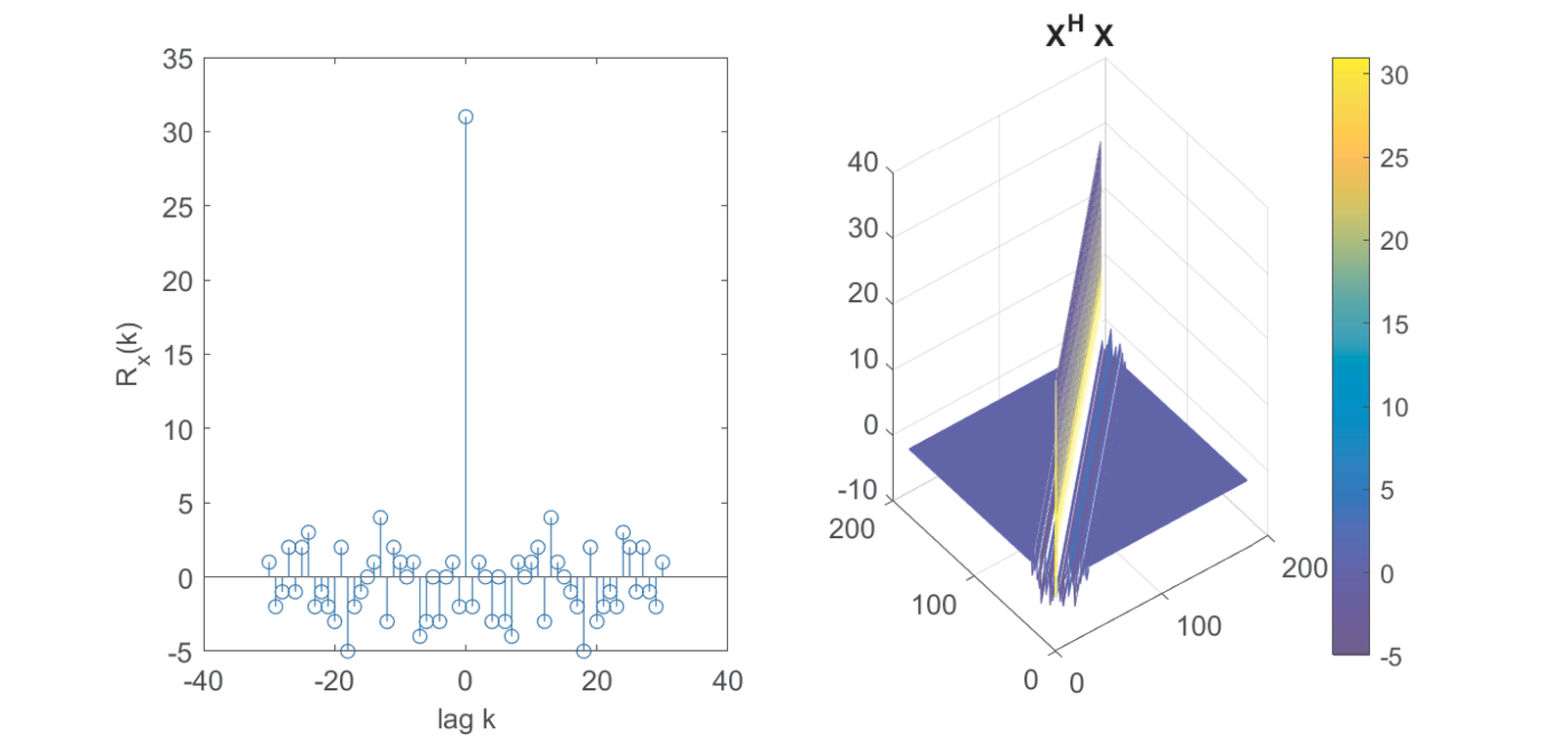
Figure 4.39 used a maximum length sequence [ url7max] or M-sequence, which are known to have an autocorrelation with a large peak. As suggested by the color bar dynamic range, the values of in Figure 4.39 coincide with and the peak value is , which corresponds to 31 in Figure 4.39.
There are alternatives to M-sequences such as the ones that have (approximately) a periodic impulse train as autocorrelation. The impulse response can be properly estimated if it fits between two impulses (i. e., there are enough zeros between them) of the autocorrelation. GSM uses such a training sequence.
Assuming that Eq. (4.41) applies, Eq. (4.39) simplifies to
|
| (4.42) |
Similar to the interpretation suggested by Figure 4.39, in Eq. (4.42) corresponds to the cross-correlation between and . To obtain synchronization, the receiver can continuously calculate this cross-correlation and search for a peak that identifies the beginning of the training sequence as seen by the receiver. After that, Eq. (4.42) can be applied to estimate the channel. A simple implementation of this procedure is discussed in the sequel.
Example 4.13. LS channel identification and synchronization. Assuming that Eq. (4.41) applies, Eq. (4.42) can be implemented as in Listing 4.9.
1h=transpose([-4+1j -3 -2-1j]) %channel, column vector
2Nh=length(h); %channel impulse response length
3Nx=15; %number of samples of training sequence
4x=mseq(2,log2(Nx+1)); %training sequence (a maximum length sequence)
5alpha=1/sum(x.^2); %1/alpha is the value of autocorrelation R(0)
6y=conv(h,x); %input signal passes through the channel
7%% Channel estimation and synchronization
8z=conv(y,flipud(x)); %use convolution to mimic correlation, or
9%alternatively, one could use z=xcorr(y,conj(x)); and to make exactly
10%equivalent to conv extract part of result: z=z(end-2*Nx-Nh+3:end);
11[maxOutput, maxIndex] = max(abs(z)); %find peak of output (R)
12h_est=alpha*z(maxIndex:maxIndex+Nh-1) %estimated channel (postcursor)
13MSE=mean(abs(h-h_est).^2) %estimation error
14NMSE=10*log10(MSE/mean(abs(h).^2)) %normalized MSE in dB
15%% Compare with theoretical values
16[R,lag]=xcorr(x); %autocorrelation. Obs: use stem(lag,R) to plot it
17z2=conv(R,h); %conceptually, this is what we are doing to get z
18z_error=max(abs(z-z2)) %note that z is equal to z2
Instead of using xcorr(x) to estimate the cross-correlation, Listing 4.9 uses convolution to obtain z. As discussed in Section E.4.3, the two alternatives are equivalent.
In the last lines, Listing 4.9 emphasizes that obtaining z2 provides an alternative interpretation of z. Using notation of sequences instead of vectors: while z was obtained with , using the commutative and associative convolution properties, the operations were rearranged to obtain z2 via , where is the autocorrelation of .
The procedure suggested by Listing 4.9 fails when the peak of the impulse response is not its first sample. For example, the reader is invited to modify Listing 4.9 to use h=[2;3;4] and observe that Listing 4.9 is restricted to extract the samples after the impulse response peak. In more elaborated schemes, after the cursor is chosen, equalizers for the pre-cursor and post-cursor parts of the channel impulse response can be used.
Example 4.14. More complete example of LS channel identification and synchronization. Listing 4.10 provides a more complete example of LS estimation. For example, it allows to investigate the impact of the AWGN SNR and input length.
1function [h,h_est,h_est2,h_est3]= ...
2    ex_systems_LS_channel_estimation(inputLengthLog2, ...
3    inputSequenceChoice, SNRdB)
4%function [h,h_est,h_est2,h_est3]= ...
5%ex_systems_LS_channel_estimation(inputLengthLog2,inputSequenceChoice)
6% inputLengthLog2=12; %the input length is 2^inputLengthLog2-1
7% inputSequenceChoice=3; %choose between following options
8% SNRdB = 20; %SNR (dB) that determines noise power. Inf is noiseless
9inputLength=2^inputLengthLog2-1; %number of input samples
10switch inputSequenceChoice %obs: input signal must be a column vector
11    case 1; x=transpose(1:2^inputLengthLog2-1); %arbitrary input
12    case 2; x=2*((rand(inputLength,1)>0.5)-0.5); %random
13    case 3; x=mseq(2,inputLengthLog2); %"maximum length" sequence
14end
15alpha = 1/sum(x.^2); %find normalization factor
16%% Define the channel. Example: a Chebyshev filter
17N=6; R=0.5; Wp=[0.3 0.5]; %order, ripple in dB and cutoff frequencies
18[B,A]=cheby1(N,R,Wp); %design filter, obs: can check with freqz(B,A)
19h=impz(B,A); %get long h (length determined by impzlength.m)
20h_power = abs(h).^2; %instantaneous power of h (assumed in Watts)
21h_totalEnergy=sum(h_power); %total energy of h (assumed in Joules)
22accumulatedEnergySum = cumsum(h_power); %accumulated sum
23energyThreshold = 99.99/100; %keep 99.99% of total energy in h
24index=find(accumulatedEnergySum > energyThreshold*h_totalEnergy,1);
25h=h(1:index); %truncated impulse response, can check with freqz(h)
26%% Pass signal through channel and add noise
27y=conv(x,h); %pass input signal through the channel
28P_receiver = mean(abs(y).^2); %power of signal of interest at Rx
29Power_noise = P_receiver / 10^(0.1*SNRdB); %noise power
30y=y+sqrt(Power_noise)*randn(size(y)); %add some noise
31X=convmtx(x,length(h)); %create convolution matrix X
32mpInv=pinv(X); %pinv is a robust estimation of the pseudoinverse
33%% Compare identification techniques:
34%1) LS estimate via Moore-Penrose pseudoinverse
35h_est = mpInv*y; %use pseudoinverse previously computed
36%2) Assuming inv(X'*X) is alpha*I  (where I is the identity matrix)
37h_est2 = alpha*X'*y; %under assumption, no need to calculate pinv(X)
38%3) Peak-searching procedure with known h peak index (hpeakIndex)
39z=conv(y,flipud(x)); %implement crosscorrelation via convolution
40[maxOutput, maxIndex] = max(abs(z)); %find peak of output (R)
41[temp, hpeakIndex] = max(abs(h)); %index of impulse response peak
42guessFirstIndex = maxIndex-hpeakIndex+1; %index to get imp. response
43h_est3=alpha*z(guessFirstIndex:guessFirstIndex+length(h)-1);%estimate
44%% Results:
45errors=[h-h_est h-h_est2 h-h_est3]; %estimation error for 3 estimates
46h_sqrt_norm=mean(abs(h).^2);
47disp(['SNR = ' num2str(SNRdB) ' dB and ' ...
48    num2str(inputLength) ' training samples'])
49disp(['NMSE: ' ...
50    num2str(10*log10(mean(abs(errors).^2)/h_sqrt_norm)) ' (dB)'])
51spectralDistort=[ak_spectralDistortion(h,h_est,length(h),10), ...
52 ak_spectralDistortion(h,h_est2,length(h),10)... %use 10 dB to get
53 ak_spectralDistortion(h,h_est3,length(h),10)]; %passband distortions
54disp(['Spectral distortions: ' num2str(spectralDistort) ' (dB)'])
Listing 4.10 also compares the solutions provided by three methods. The first one corresponds to using Eq. (4.39) and the other two to Eq. (4.42), which assume that Eq. (4.41) applies. The third method differs from the previous two because it does not assume complete knowledge about synchronization. Also, there are three different options for the training sequence. For example, using inputSequenceChoice=1 makes the second and third estimation methods fail because Eq. (4.41) would not be observed.
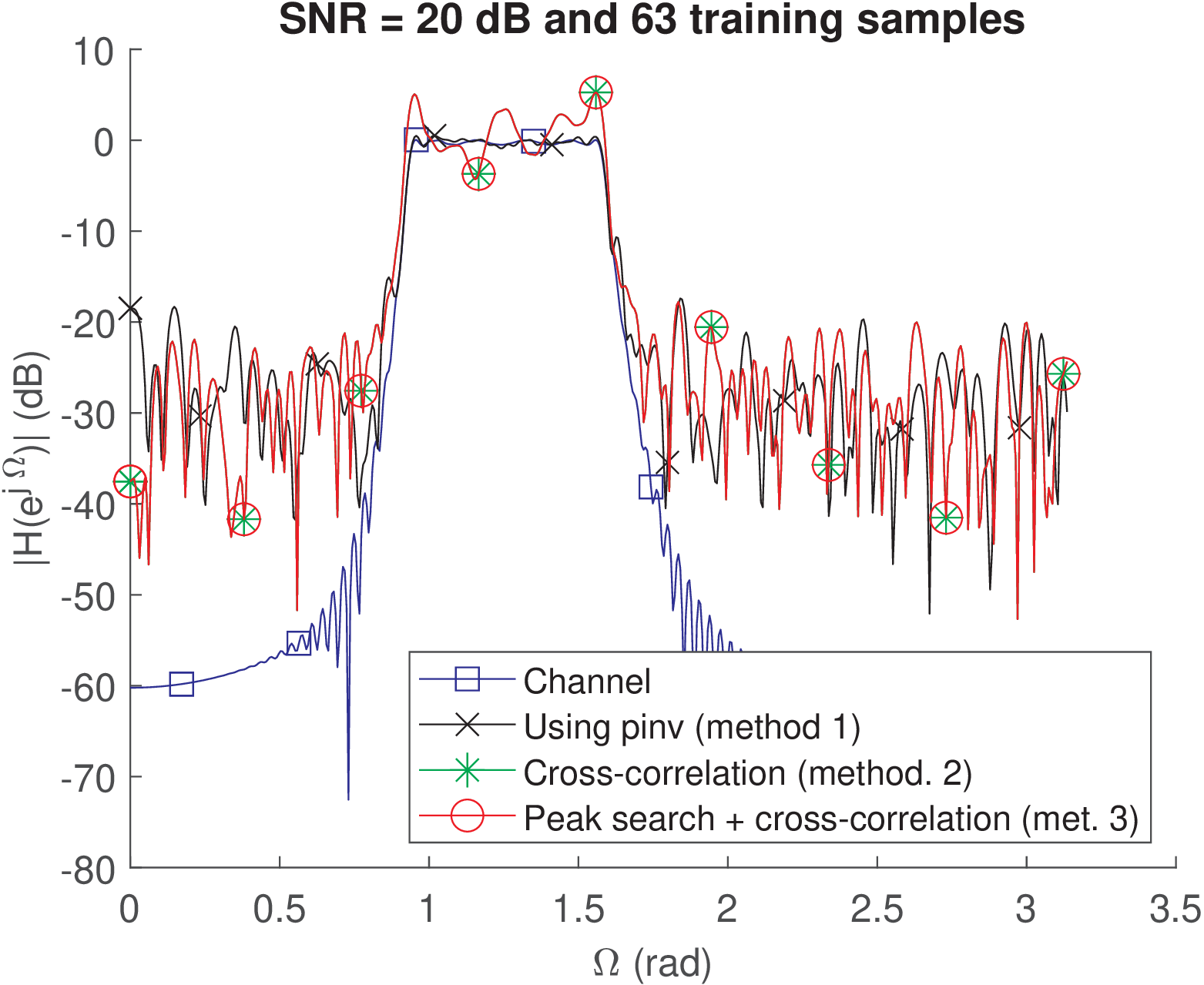
Figure 4.40 shows a plot obtained after running Listing 4.10 with inputs inputLengthLog2=6, inputSequenceChoice and SNRdB = 20. The channel is a bandpass Chebyshev type I filter, the SNR is 20 dB and the input is an M-sequence (inputSequenceChoice=3) with samples. In this case, the comparisons between the correct h and the estimates h_est, h_est2 and h_est3 leads to, respectively (results may slightly change due to the random number generators):
     SNR = 20 dB and 63 training samples
     NMSE: -18.7647     -7.05488     -7.05488 (dB)
     Spectral distortions: 0.12043      1.2796      1.2796 (dB)
The second and third methods obtained the same result because the “synchronization” worked properly in this case, and guessFirstIndex was indeed the best option. The first method significantly outperforms the others because the training sequence is relatively short and Eq. (4.41) is not accurate. The average spectral distortion over the passband13 increased from 0.12043 to 1.2796 dB when going from method 1 to 2 (or 3). In fact, as illustrated in Figure 4.40, the frequency response estimated by the two latter methods have peaks of more than 3 dB over the passband.
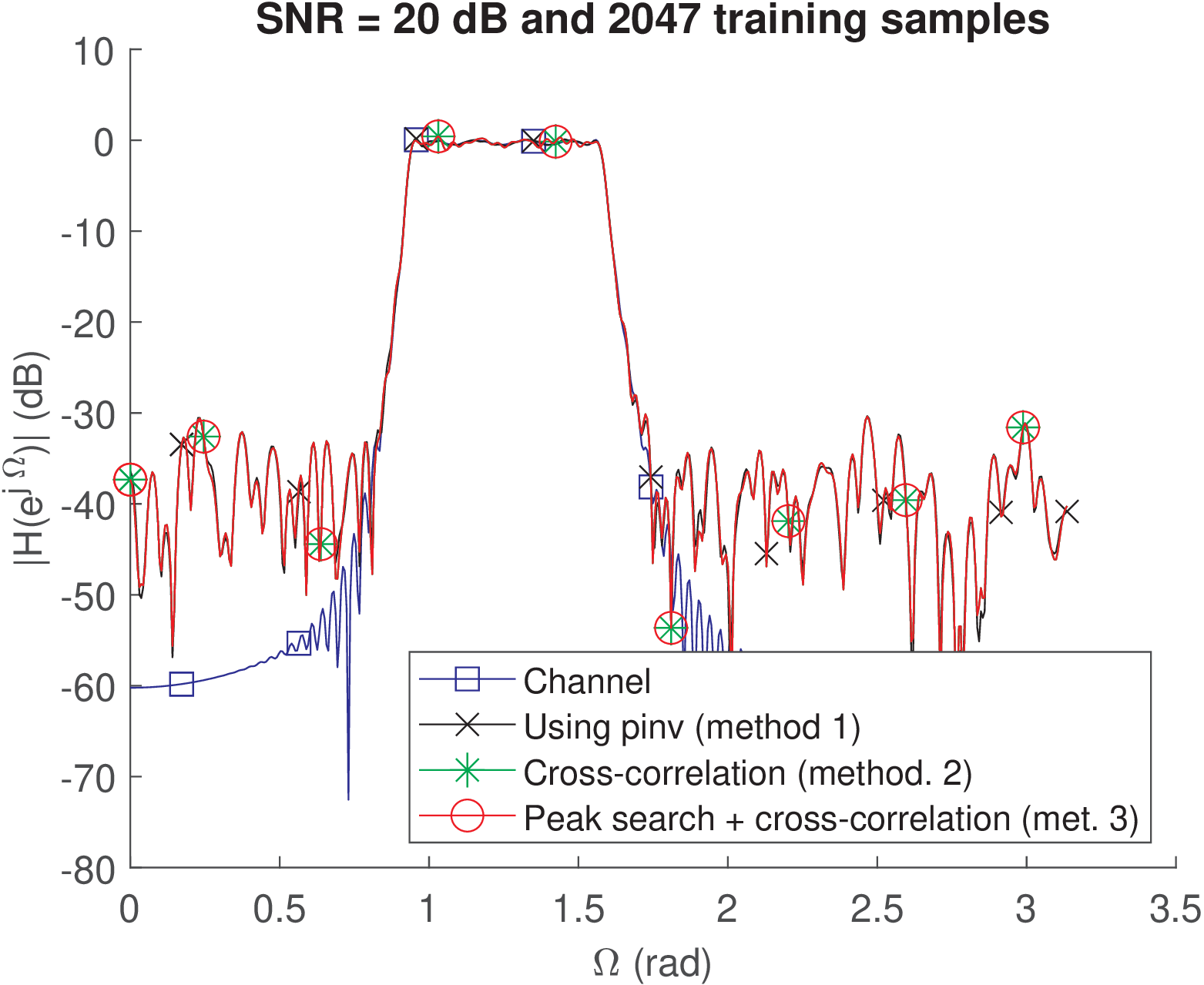
Increasing the training sequence length from 63 to 2047 samples (by changing inputLengthLog2 from 6 to 11) leads to Figure 4.41 and the following result:
     SNR = 20 dB and 2047 training samples
     NMSE: -30.767     -26.1736     -26.1736 (dB)
     Spectral distortions: 0.035982      0.1119      0.1119 (dB)
In this case, a relatively long M-sequence is used and all three methods had performance limited by the SNR. The longer training sequence leads to a better approximation of Eq. (4.41) for Methods 2 and 3. The average spectral distortion of all three methods was below 1 dB over the passband.
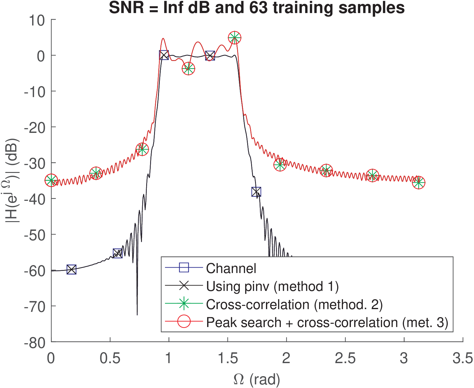
Using a training sequence length of 63 and infinite SNR leads to Figure 4.42 and the following result:
     SNR = Inf dB and 63 training samples
     NMSE: -292.1716     -7.321442     -7.321442 (dB)
     Spectral distortions: 3.5922e-15      1.2649      1.2649 (dB)
In this case, the first method obtained h_est virtually equals to h, where the NMSE of dB indicates there were only numerical errors. However, the other two methods did not improve given that the training sequence is relatively short.
Note that synchronization was not a problem even for method 3. In case, guessFirstIndex were not the best option, method 3 would be outperformed by method 2. In fact, it is not trivial to implement Eq. (4.42) and better algorithms than the ones in Listing 4.10 should be used to achieve a more robust estimation in practice. This issue is further discussed in Application 4.6 in the context of GSM.
Given that the channel has been estimated with LS or other method, it remains the task of designing the equalizer. The next subsection discusses one well-known criterion.
4.9.2 Zero-forcing (ZF) equalization criterion
When dealing with a frequency-selective channel , it is tempting to use an equalizer to try to completely remove any effect of . Theoretically, this is possible using an equalizer designed with the zero-forcing criterion. If is the Laplace transform of , the zero-forcing equalizer (ZFE) corresponds to a system function . However, if at some value , then , which creates problems in practice. For example, for all frequencies larger than the cutoff frequency of the ideal lowpass filter, even with an infinite gain, the equalizer cannot recover the input signal because the components with frequency were already zeroed. But the ZF criterion does not capture this condition and would still try to invert the channel.
Another aspect is that the zeros in become the poles in the ZFE. Hence, if is minimum phase, i. e., its inverse is causal and stable. For example, assuming causal systems, if all the zeros of are at the left-half side of the the -plane, then the equalizer is stable. But if the channel is not minimum phase, the ZFE may be unstable (or noncausal). Similarly, for discrete-time and causal signals, zeros of outside the unit circle would lead to an unstable ZFE system .
Example 4.15. Impact of minimum phase in equalization. Listing 4.11 creates a minimum phase discrete-time channel and the function deconv can perfectly recover the channel input signal:
1zeros=[0.3*exp(j*pi/2) 0.3*exp(-j*pi/2) ...
2 0.8*exp(j*pi/4) 0.8*exp(-j*pi/4)];
3h=poly(zeros);
4n=0:1000-1; %abscissa
5x=4*cos(pi/8*n) + 6*cos(0.7*pi*n+pi/5); %input signal
6y=conv(x,h); %filter
7xRecovered=deconv(y,h); %try to deconvolve
8plot(x-xRecovered) %compare the signals
In contrast, the FIR filter designed with Listing 4.12 has zeros [-16.79 -1.0 -0.06] and, therefore, is not minimum phase as can be seen with the command zplane(h).
1N=3; %filter order
2fc=0.4*pi; %cutoff frequency (rad)
3h=fir1(N,fc/pi); %design lowpass filter
4n=0:1000-1; %abscissa
5x=4*cos(pi/8*n) + 6*cos(0.7*pi*n+pi/5); %input signal
6y=conv(x,h); %filter
7xRecovered=deconv(y,h); %try to deconvolve
Observing the signal xRecovered shows that it diverges and has amplitudes going to infinite.
In practice, the equalizer should work only for frequencies within the channel passband. Hence, one important requirement is to design the communication system such that the transmitted signal has a PSD with most of its power contained within the system bandwidth. This allows the receiver to, taking that in account, filter the out-of-band signal and equalize within the frequency band of interest.
One of the most used ZFEs are the discrete-time FIR equalizers estimated via least squares. This specific class of equalizers will be discussed in the sequel.
4.9.3 Least squares FIR equalizer based on estimated channel
Assuming estimated channel FIR coefficients stored in vector , the ZFE would be an IIR filter. However, it is sometimes advantageous to also use a FIR to perform equalization due to properties such as stability and simpler design. In the sequel, the least squares (LS) method is used to design a FIR equalizer .
Denoting the elements of and as sequences and , the ZF criterion suggests seeking that leads to , where is the delay the signal suffers after passing through the (estimated) channel and equalizer. The design of can be cast as a LS problem written in matrix notation as
|
| (4.43) |
where is the convolution matrix obtained from and is a vector with zeros but the -th element, which is one, representing .
Similar to Eq. (4.37) and its solution Eq. (4.39), the solution to Eq. (4.43) uses the pseudoinverse and is given by
|
| (4.44) |
with a corresponding MSE given by .
The optimal value of in Eq. (4.44) depends on and can be found by trial-and-error.14 An educated guess can be , where is the number of rows of (i. e., the number of elements in the convolution output). The number of elements of is also , such that the suggested guess corresponds to positioning the impulse approximately in the middle of .
Example 4.16. Least squares equalizer. Listing 4.13 provides an example of using Eq. (4.39) to design an equalizer.
1rng('default'), rng(10); %set a seed
2Nw=10; %number of equalizer coefficients
3h=[5.1; 0; 0; 0.5; 3; 0.2; -0.1]; %channel impulse response
4Nh=length(h); %number of impulse response coefficients
5Hhat=convmtx(h,Nw); %convolution matrix. Note that Hhat*w = conv(w,h)
6Nc=Nw+Nh-1; %number of elements in convolution output
7MSEvalues=zeros(Nc,1); %pre-allocate space
8for Delta=1:Nc %search for best delay Delta
9    e=zeros(Nc,1); e(Delta)=1; %create vector to mimic impulse
10    w=pinv(Hhat)*e; %find the equalizer
11    %w2=inv(Hhat'*Hhat)*Hhat'*e; %use pseudoinverse property
12    %max(abs(w-w2)) %compare with pinv
13    MSEvalues(Delta)=mean(abs(Hhat*w - e).^2); %calculate MSE
14end
15stem(1:Nc,MSEvalues), xlabel('delay \Delta'), ylabel('MSE') %plot
16[minMSE,bestDelta]=min(MSEvalues) %find best delay and its MSE
17guessBestDelta=round((Nc-1)/2) %guess best delay value
18e=zeros(Nc,1); e(bestDelta)=1; %create vector with best delay
19wbest=inv(Hhat'*Hhat)*Hhat'*e; %best equalizer
20%% Check equalization performance
21stem(e), hold on, stem(conv(h,wbest),'r')
The output of Listing 4.13 with Nw=10 and h=[0.1; 0; 0; 0.5; 3; 0.2; -0.1] is:
minMSE = 2.9126e-07 bestDelta = 11 guessBestDelta = 8
which indicates that the best was 11, with a , while rounding suggested . The reader is invited to vary Nw and/or h, observing how the performance changes. For example, one obtains
minMSE = 0.0022 bestDelta = 2 guessBestDelta = 8
when keeping Nw=10 and modifying the first element of h from 0.1 to 5.1.
4.9.4 FIR equalizer: LS direct estimation with training sequence
Eq. (4.37) and Eq. (4.43) can be depicted via block diagrams as follows:
|
| (4.45) |
and
|
| (4.46) |
respectively. In both cases, the sequence within the boxes should be estimated.
Instead of first estimating the channel and then the equalizer, it is often more convenient and accurate to directly obtain the equalizer. As previously, the LS solution can be obtained by solving a set of linear equations.
The LS equalizer can be obtained directly by considering as goal to implement:
|
| (4.47) |
where should be estimated to transform the observed received signal back into the training sequence , according to the ZFE criterion.
The equivalent system is and the LS solution uses the pseudoinverse given by
|
| (4.48) |
where is the training sequence.
Example 4.17. Least squares equalizer. Listing 4.14 provides an example of using Eq. (4.48) to design an equalizer.
1rng('default'), rng(10); %set a seed
2Nw=5; %number of equalizer coefficients
3h=[0.1; 0; 0; 0.5; 3; 0.2; -0.1]; %channel impulse response
4x=transpose(1:11); %arbitrary training sequence as column vector
5Nx=length(x);
6if Nw >= Nx
7    error('System should be overdetermined. Use Nw < Nx')
8end
9y=conv(x,h); %convolve input with channel impulse response
10Ycomplete=convmtx(y,Nw); %complete convolution matrix
11%Ycomplete=convmtx(transpose(1:Ny),Nw) %complete convolution matrix
12[Ny temp]=size(Ycomplete); %Ny=Nx+length(h)+Nw-2, result of 2 conv's
13MSEvalues=zeros(Ny-Nx+1,1); %pre-allocate space
14for Delta=1:Ny-Nx+1 %Ny-Nx+1 %search for best delay Delta
15    Yhat=Ycomplete(Delta:Delta+Nx-1,:); %delayed convolution matrix
16    w=pinv(Yhat)*x; %find the equalizer
17    %w2=inv(Yhat'*Yhat)*Yhat'*x; %design using the property
18    %max(abs(w-w2)) %compare with pinv
19    MSEvalues(Delta)=mean(abs(Yhat*w - x).^2); %calculate MSE
20end
21stem(1:Ny-Nx+1,MSEvalues), xlabel('delay \Delta'), ylabel('MSE')%plot
22[minMSE,bestDelta]=min(MSEvalues) %find best delay and its MSE
23Yhat=Ycomplete(bestDelta:bestDelta+Nx-1,:); %convolution matrix
24wbest=pinv(Yhat)*x; %find the equalizer
25%wbest2=inv(Yhat'*Yhat)*Yhat'*x; %find the equalizer
26%% Check equalization performance
27stem(conv(h,wbest))
The output of Listing 4.14 is:
minMSE = 1.4257e-06 bestDelta = 11
Decreasing Nw from 10 to 5 increases minMSE to .
4.9.5 Probabilistic approach to LS FIR system identification
The previous discussion has concentrated on deterministic signal processing, but a probabilistic approach is more suitable in scenarios involving random processes. One specific formulation for channel identification is briefly presented in the sequel.
The correlation matrix of can be defined as
|
| (4.49) |
and the cross-correlation as
|
| (4.50) |
Using these definitions, Eq. (4.39) can be written as
|
| (4.51) |