4.10 Channel Capacity
The channel capacity is the maximum rate of communication for which an arbitrarily small error probability can be achieved. It is an intrinsic property of a channel and extensively studied in the Information Theory literature.
Each channel has its capacity and this concept gets confused because sometimes the word capacity is also used to describe the bit rate achieved by a given communication system. For example, under this alternative interpretation of “capacity”, one can say that increasing the number of bits per symbol a PAM from to 4 doubled the “capacity”. This terminology should be avoided and, instead, bit rate used in this case.
Because each channel has its capacity, a given expression for capacity must be used only for the specific channel that it was derived for.
4.10.1 Capacity of AWGN channels
In the case of the continuous-time AWGN channel of Figure 4.6, the capacity in bits per second (bps) is15
|
| (4.52) |
where is given in Hz and is the SNR at the receiver, in linear scale (not dB).
Recall from Section 4.2.5, that the transmit signal power of an AWGN channel is power-limited. This avoids the situation of having an infinite capacity by increasing the SNR in Eq. (4.52). In practice, is finite because the transmit signal power is always bounded and the noise power is not zero.
From Eq. (4.52), it can also be seen that doubling leads to twice the capacity, but the dependence of on is only logarithmic.
The discrete-time AWGN channel does not have any time explicitly associated to the transmission of a vector of dimension and one cannot specify the symbol duration in seconds, for example. Hence, it is more sensible to account capacity as bits “per channel use” (bpcu) or “per transmission” in this case, where each “use” is the transmission of a vector with symbols. For example, and 2 when using PAM and QAM, respectively. Assuming that the unit is “bits per channel use per dimension”, the normalized capacity of the discrete-time AWGN channel is
|
| (4.53) |
and its total capacity bits per channel use.
Eq. (4.53) is also called the capacity of the discrete-time real AWGN, while the capacity of the complex version (that corresponds to using QAM instead of PAM) is
|
| (4.54) |
Note that Eq. (4.52) is valid for both real and complex AWGN channels, and it can be obtained from Eq. (4.53) or Eq. (4.54) as follows. When the symbols are real-valued (e. g., when PAM is used in baseband channels), Table 4.2 indicates that the maximum number of symbols that can be sent over a channel with bandwidth BW is . Therefore, using Eq. (4.53), the capacity is
as indicated by Eq. (4.52). Similarly, when the symbols are complex-valued (e. g., when QAM is used in bandpass channels), Table 4.3, indicates that the maximum number of symbols that can be sent over a channel with bandwidth BW is and from Eq. (4.54):
4.10.2 Water filling
This section discusses the water filling (or water pouring) algorithm that provides the optimum allocation of power in order to achieve the capacity of the frequency-selective channel depicted in Figure 4.1. A by-product of using water filling for power allocation is an estimate of the channel capacity itself. It is assumed that the transmit signal is constrained to have a maximum power value (otherwise the capacity would be infinite).
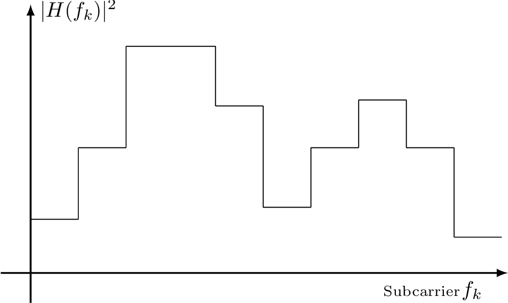
The strategy to achieve the capacity in this case is to segment the available BW into “subchannels” with small BW denoted as , such that the gain can be assumed constant within . With this strategy, the frequency-selective channel is transformed into a set of parallel “subchannels”, with each one modeled as AWGN with a frequency response magnitude that is flat over frequency, as depicted in Figure 4.43(a). More specifically, the -th “subchannel” has a center frequency corresponding to a subcarrier or tone, and frequency response that is assumed flat, as depicted in Figure 4.2. For convenience, the squared magnitude is denoted as .
(a)
Channel
gains. |
(b)
Water
filling
solution. |
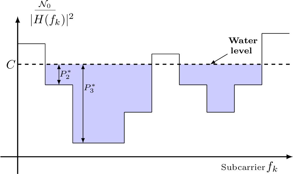
Assuming the WGN at the receiver has a unilateral PSD value of , the noise power on each “subchannel” is
|
| (4.55) |
To achieve capacity, the total transmit power needs to be distributed among the subcarriers such that . This power allocation problem does not appear in the AWGN of Figure 4.6. Figure 4.43(b) indicates the solution, which is known as “water filling”, and provides the optimum power value as
|
| (4.56) |
where is known as the “water level”. If the first argument of the max function in Eq. (4.56) is negative, and no power is allocated to transmission using the -th subcarrier.
The water filling solution will be further discussed in the sequel, but note that after the optimum power allocation is obtained, Eq. (4.53) can be used to calculate the total capacity in bits per channel use as
|
| (4.57) |
where is the SNR at subcarrier . It is assumed in Eq. (4.57) that each subcarrier uses dimensions.
Eq. (4.57) can be converted to bits per second, by taking in account that each subchannel has a bandwidth . Using and Eq. (4.57), the capacity of the parallel channels is
|
| (4.58) |
Assuming that is the PSD value of the received signal (after passing the channel), which can be assumed16 constant over , is the ratio between the received power and the noise power , which can be simplified to
|
| (4.59) |
Eq. (4.59) indicates that, instead of using power values, can be obtained from the associated PSD values given that is canceled out.
The PSD at the transmitter can be taken in account via Eq. (F.40), which allows to write . Hence, the SNR in terms of the transmit PSD, channel response and noise at receiver is
|
| (4.60) |
Substituting Eq. (4.60) into Eq. (4.58) leads to
|
| (4.61) |
where denotes the optimum transmit PSD.
Water filling for a finite set of parallel channels
As mentioned, the optimum solution to the power loading problem is the water filling. More specifically, the power loading problem is the following: maximize Eq. (4.57) subject to a maximum transmit power . The problem is convex and can be solved using a Lagrange multiplier. The optimality relies on the fact that Eq. (4.57) is a convex (in fact, concave) function of the PSD, which influences the SNR according to Eq. (4.60). Before delving in the the associated mathematics, a very simple example of water filling will be described.
Example 4.18. Power loading with only two tones. The problem here is to allocate power considering that there are only parallel channels. At the tones and 1, the channel has squared magnitude and , respectively. The number of channel uses per second is kbauds and kHz is adopted. The background noise is modeled as having a white (unilateral) PSD with dBm/Hz, which corresponds to W/Hz and a noise power of W per tone. It is assumed that both tones can use and transmit QAMs. The maximum transmit power is 1 mW, such that mW. Figure 4.44 shows the rate for each pair . Figure 4.44 indicates that the rate obtained with Eq. (4.57) is a concave function of the PSD.
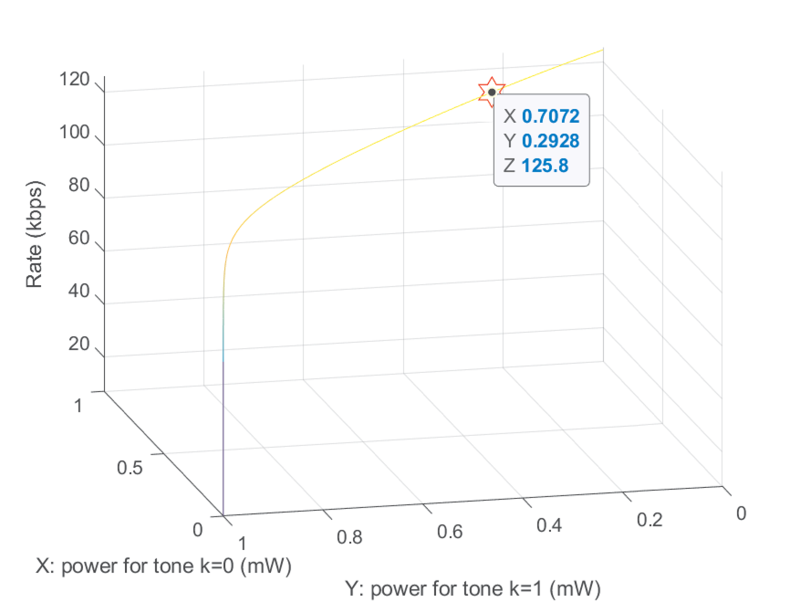
When all the power is allocated to the worst tone , the total rate is only kbps. When the total power is allocated to , the rate is 124.7 kbps. The best allocation is mW and mW, which achieves kbps, as indicated in Figure 4.44 by the marker. The main point here is to observe that convexity can be assumed and this enables easier procedures to find the optimum solution.
Watefilling solution via Lagrange multiplier
Given that Eq. (4.57) is convex, it is possible to maximize it using a Lagrange multiplier to constrain the total power. Hence, the Lagrangian can be formulated as
For a specific subchannel , calculating decouples from the tones as follows:
which can be simplified to
|
| (4.62) |
Hence, the solution, which was anticipated in Eq. (4.56) is to pour power according to the transmit PSD (“water”) on a curve specified by , which can be seen as an “inverse SNR” such that the summation of these two parcels corresponds to the water level , which is the same for all tones and needs to be found by the algorithm. Listing 4.15 lists the first lines of a simple water filling algorithm.17 The fourth parameter (gap) of ak_simplewaterfill will be discussed in Section 5.8 and its default value can be assumed here.
1function [powerPerTone,powerWaterlevel,SNR] = ...
2    ak_simplewaterfill(g,noisePowerPerTone,totalPower,gap)
3% Inputs:
4%  g - squared magnitude of the channel frequency response
5%  noisePowerPerTone - noise power per tone (scalar array
6%                     with the same dimension of g)
7%  totalPower  total power (or energy)
8%  gap - gap (not in dB, but linear scale). Default value is 1
9% Outputs:
10%  powerPerTone - optimum power allocation per tone
11%  waterlevel - power (not PSD) level of the water filling
12%  SNR - signal to noise ratio in linear scale (not dB)
13% It assumes all the channels are of the same type (e.g.
14% PAM or QAM) and have the same dimension (1 or 2)
With the help of ak_simplewaterfill.m (Listing 4.15), the solution that maximizes rate in Figure 4.44 can be easily obtained with Listing 4.16.
1g=[0.1 1e-10]; %channel squared magnitudes
2deltaf = 4.13125e3; %subchannel BW (borrowed from ADSL standard)
3N0 = 1e-17; %noise PSD in Watts/Hz, corresponding to -140 dBm/Hz
4noisePowerPerTone = N0 * deltaf; %noise power at each tone
5totalPower=1e-3; %total power (Watts) to be shared between tones
6[powerPerTone,waterlevel,SNR]=ak_simplewaterfill(g,...
7  noisePowerPerTone,totalPower) %solution provided by waterfilling
8bitsPerTone = log2(1 + (powerPerTone.*g)/noisePowerPerTone) %bits
Note that water filling in Listing 4.16 provided 0.706562 and 0.29344 mW as the optimum power allocation, which is slightly different (and better) than the values in Example 4.18. The reason is that Example 4.18 used a discrete grid to search for the optimum and the grid resolution did not allow to find it exactly.
Example 4.19. Another example of water filling. For another water filling example, consider the conversion of a channel into a set of parallel channels with squared magnitudes . The total power is W. Assuming the unilateral white noise PSD has value W/Hz, and the subchannel BW is kHz, the noise power at each tone is W. The script MatlabOctaveBookExamples/ex_channel_waterfill.m was used with these values to obtain Figure 4.45.
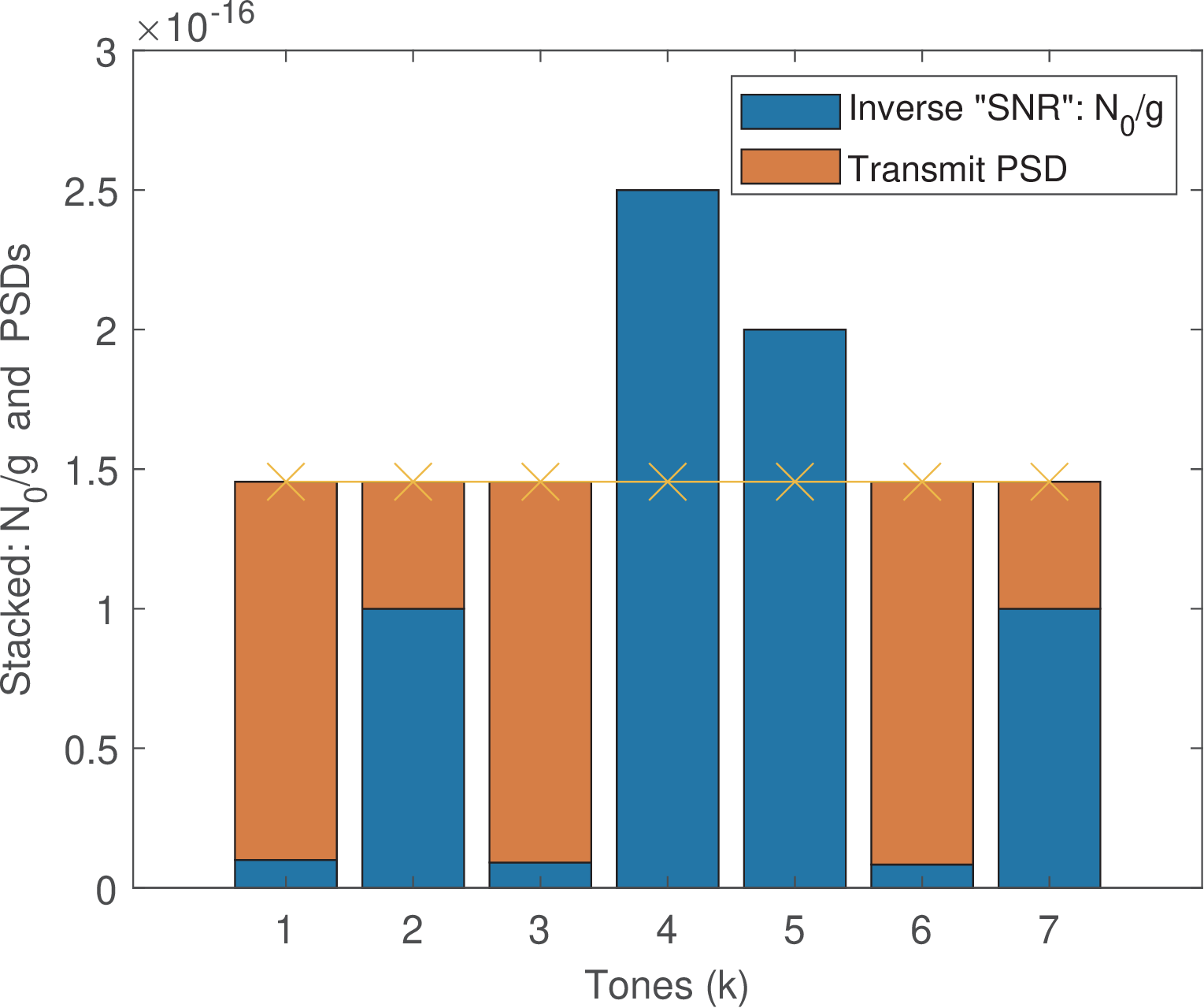
As indicated in Figure 4.45, the water level in this case is . The optimum PSD is S.
Power was not allocated to tones 4 and 5 due to their being higher than . Most of the power is allocated to tones 1, 3 and 6, due to their relatively high gains. In this case, the SNR per tone is in linear scale and, assuming dimensions can be used, the capacity is 13.07 bits per channel use.
After a channel is partitioned in parallel channels and the available power is distributed among these channels, Eq. (4.53) or Eq. (4.54) can be used to determine their capacities. The capacity can then be used to estimate the (maximum) bit rate.
The power loading problem is related to the bit loading problem, as will be discussed in Chapter 6. Often the number of bits (constellation cardinality) must be integer valued.18 In this case, simply using a continuous water filling algorithm for power loading, and then truncating (or rounding) the number of bits provided by capacity equations leads a simple but suboptimal solution.19
Water filling for continuous frequency
The capacity of a frequency selective LTI Gaussian channel with frequency response and bandwidth BW is also achieved with a water filling solution, but now in a continuous frequency . This water filling can be obtained by letting the number of subchannels go to infinite, which makes the bandwidth of each subchannel go to zero. Eq. (4.56) then converges to
|
| (4.63) |
where the water level is chosen such that
|
| (4.64) |
and is the optimum transmit PSD.
4.10.3 Capacity of the frequency-selective LTI Gaussian channel
Using the optimum PSD provided by Eq. (4.63), the capacity of the frequency-selective LTI Gaussian channel in bits per second is then
|
| (4.65) |
Eq. (4.65) can be obtained from the capacity expression from a set of parallel channels and making . More specifically, substituting into Eq. (4.61), leads to
|
| (4.66) |
which converges to Eq. (4.65) when and the discrete frequencies become to describe a continuous frequency response .
4.10.4 Revisiting the capacity of flat fading continuous-time AWGN
Note that the channels in Figure 4.6, with a flat frequency response, can be seen as special cases of the frequency-selective LTI Gaussian channel. Applying water filling as in Eq. (4.63) to the channels in Figure 4.6 would lead to flat transmit PSDs with BW, where is the maximum transmit power (unilateral PSDs are adopted). Using Eq. (F.40), the PSD at the receiver is , where is the frequency response magnitude over the channel passband. Hence, the SNR at the receiver is
|
| (4.67) |
Substituting Eq. (4.67) into Eq. (4.52) leads to
|
| (4.68) |
Hence, only when the channel is frequency-selective the water filling solution is required for obtaining the optimum transmit PSD and, from that, the channel capacity. Alternatively, Eq. (4.68) suffices to calculate the capacity for channels with flat frequency responses.
Example 4.20. Example of capacity calculation for a continuous-time AWGN channel. Assume that the bandpass channel depicted in Figure 4.6(b) has Hz and magnitude over the passband. The WGN has a unilateral PSD level mW/Hz and the maximum transmit power is mW.
Using Eq. (4.68), the capacity of this channel is
For practicing the interpretation of Eq. (4.61), consider that the current channel is modeled as a set of subchannels, each with Hz. Because the channel is flat, the water filling solution would equally split among the four subchannels, with mW being allocated to each, corresponding to a PSD level of mW/Hz, . In this case, the capacity per channel use of a subchannel is
which leads to
which coincides with the result from Eq. (4.68).