5.8  The Gap Approximation

The next sections discuss the so-called gap approximation applied to PAM and QAM.

5.8.1  The PAM 6-dB rule: each extra bit requires 6 dB

An interesting relation obtained from Eq. (5.8) is

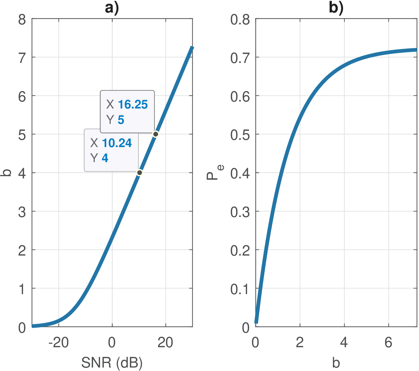
Figure 5.16 a) presents a graph of Eq. (5.17) when varying $\mathrm{\text{SNR}}$ for ${\sigma }^2=\; 2$ and $d\; =\; 1$. It indicates that, when $b$ is sufficiently high, each additional bit (from 4 to 5 bits, for example) requires an increase of 6 dB in SNR if one desires to maintain the $P_e$. Another way of observing this fact is to assume that $12\frac{\mathrm{\text{SNR}}{\sigma }^2}{d^2}»\; 1$ and obtain

which can be expressed as $\mathrm{\Delta }b\; \approx \; 0.1661\mathrm{\Delta }{\mathrm{\text{SNR}}}_{\mathrm{\text{dB}}}$ or $\mathrm{\Delta }{\mathrm{\text{SNR}}}_{\mathrm{\text{dB}}}\approx \; 6.0206\mathrm{\Delta }b$.

Figure 5.16 b) indicates how $P_e$ varies with $b$, which was allowed to assume non-integer values. Because ${\sigma }^2$ and the separation $d$ among symbols is kept constant, the parcel $Q\left(d∕(2\sigma )\right)$ is constant and, in this case, approximately 0.36. Hence, $P_e$ tends to $2\; \times \; 0.36$ as $b$ increases.

It is important to understand that, in spite of Eq. (5.17) looking like the “capacity” equation, this expression does not say anything about probability of error nor if this number $b$ of bits is below or above the capacity $\overline{C}=\frac{1}{2}{log}_2\left(1\; +\mathrm{\text{SNR}}\right)$ (Eq. (4.53), repeated here for convenience) of a discrete-time AWGN channel.

We are interested in understanding the gap approximation for uncoded PAM and QAM:

This approximation is widely used and the reason is the following task: say one has an estimated SNR (or, equivalently, $E_c$ and ${\sigma }^2$) and wishes to find $b$ to operate at a given $P_e$. In other words, some function $b\; =\; f(P_e,\mathrm{\text{SNR}})$ is needed.

In this situation, one does not know $b$, $M$ or $d_{min}$ that allows to achieve the target $P_e$. Hence, Eq. (5.17) cannot be used. The capacity

only tells the theoretical (assuming the possibility of infinite delay and complexity) maximum value of $\overline{b}$, but does not indicate the probability of error when using an uncoded PAM and QAM (or any other code). However, one can use expressions for $P_e$ that take into account SNR and $b$. In the following paragraph, PAM is assumed, but a similar reasoning applies to QAM.

For PAM, one has

However, because $M$ (and, equivalently, $b\; ={log}_{2}M$) cannot be expressed in closed form, it is not possible to find an “inverse” $b\; =\; f(P_e,\mathrm{\text{SNR}})$. Two alternatives are to plot the expression for $P_e$ or even find $M$ numerically. More commonly, one adopts the “gap approximation” that (in this case) consists in ignoring the term $(2∕M)Q\left(\sqrt{\frac{3}{M^2-1}\mathrm{\text{SNR}}}\right)$ and adopt:

Figure 5.17 illustrates the approximation for $\mathrm{\text{SNR}}=\; 10$ dB, where it can be seen how the discarded term $P_e-{\widehat{P}}_e=\; (2∕M)Q\left(\sqrt{\frac{3}{M^2-1}\mathrm{\text{SNR}}}\right)$ varies with $b$.

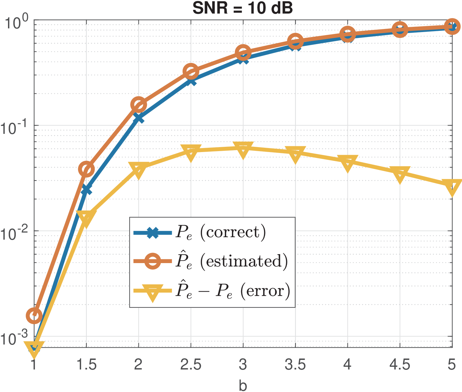
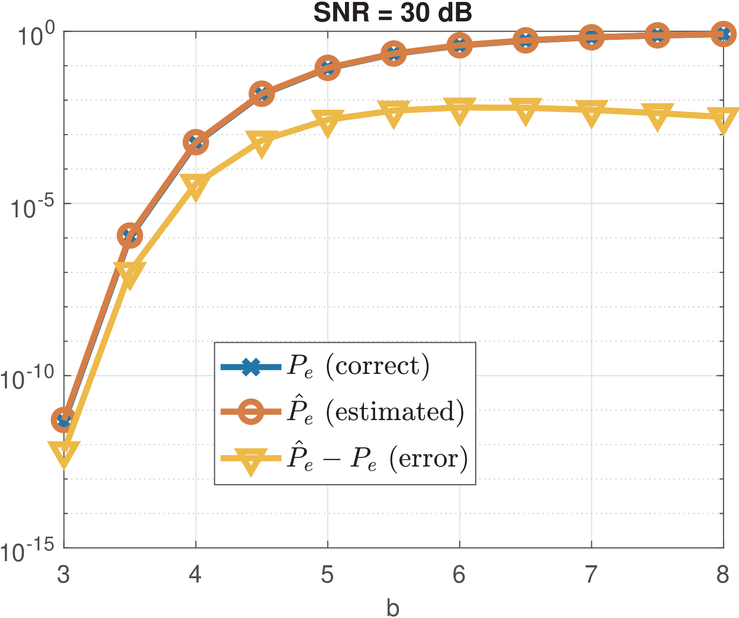
Figure 5.18 is similar to Figure 5.17 but adopts $\mathrm{\text{SNR}}=\; 30$ dB. Note that the gap approximation improves when the SNR increases.

Assuming the gap approximation of Eq. (5.19), to find $M$ that corresponds to the desired $P_e$, one can now simply isolate $M$:

and write

where

is the gap for PAM in linear scale.

5.8.2  The QAM 3-dB rule: each extra bit requires 3 dB

An expression can be derived for the number of bits per dimension of a SQ QAM:

In this case, $D\; =\; 2$, and $b\; =\; 2\overline{b}$ such that $\mathrm{\Delta }{\mathrm{\text{SNR}}}_{\mathrm{\text{dB}}}\approx \; 3.0103\mathrm{\Delta }b$ for QAM. This expression is similar to Eq. (5.17).

For square QAM, one has

In this case, the gap approximation is based on the assumption that

which allows to write

and, alternatively

where

is the gap for square QAM.

In summary, the actual supportable bit rate at a given error rate for uncoded QAM and PAM is given by the channel capacity for a modified SNR, which is the “capacity” SNR divided by the so-called SNR gap. The notion of a “gap” is more appropriate when the SNR is given in dB, since the SNR gap is then a fixed additive term for a given error rate:

Note from Eq. (5.20) and Eq. (5.23) that the gap is independent of the number of bits $b$, (and so independent of $M$ for $M$-QAM). It purely depends on the error rate.

Listing 5.8 was used to obtain Table 5.2.

1Pe = [2e-5 1e-5 2e-6 1e-6 2e-7 1e-7 2e-8 1e-8 2e-9 1e-9]; 
2argQ_qam = qfuncinv(Pe/4); %QAM 
3gap_linear_qam = (argQ_qam.^2)/3; 
4gap_db_qam = 10*log10(gap_linear_qam); 
5argQ_pam = qfuncinv(Pe/2); %PAM 
6gap_linear_pam = (argQ_pam.^2)/3; 
7gap_db_pam = 10*log10(gap_linear_pam);

For example, assume a QAM that operates with $\mathrm{\text{SNR}}=\; 20$ dB ($100$ in linear scale) and must have a symbol error rate $P_e=\; 2\; \times \; 10^{-6}$. According to Table 5.2, in this case the gap is $\Gamma \; =\; 7.976$, which leads to

Using Eq. (5.22), one obtains $P_e\approx \; 2\; \times \; 10^{-6}$ as desired. Recalling that the quantities per dimension for QAM are ${\overline{P}}_e=P_e∕2$ and $\overline{b}=\; b∕2$, the same project can be done evaluating a PAM for each dimension. In this case, ${\overline{P}}_e=\; 10^{-6}$ and, for PAM, $\Gamma \; =\; 7.976$, such that:

and, using Eq. (5.19), ${\overline{P}}_e=\; 10^{-6}$. This corresponds to $b\; =\; 2\overline{b}=\; 3.6865$ bits and $P_e=\; 2\; \times \; 10^{-6}$, as expected. Therefore, Eq. (5.18) is valid for both PAM and squared QAM.

Figure 5.19 was obtained with SNR = 10 dB for QAM. The abscissa informs the $P_e$ that was specified and the “correct” graph corresponds to $b$ using Eq. (5.21) while the other graph uses Eq. (5.23) to calculate $\Gamma$ and then $\widehat{b}$ using Eq. (5.18). It can be noticed that the number $\widehat{b}$ of bits to achieve the specified $P_e$ is underestimated by the gap approximation ( .

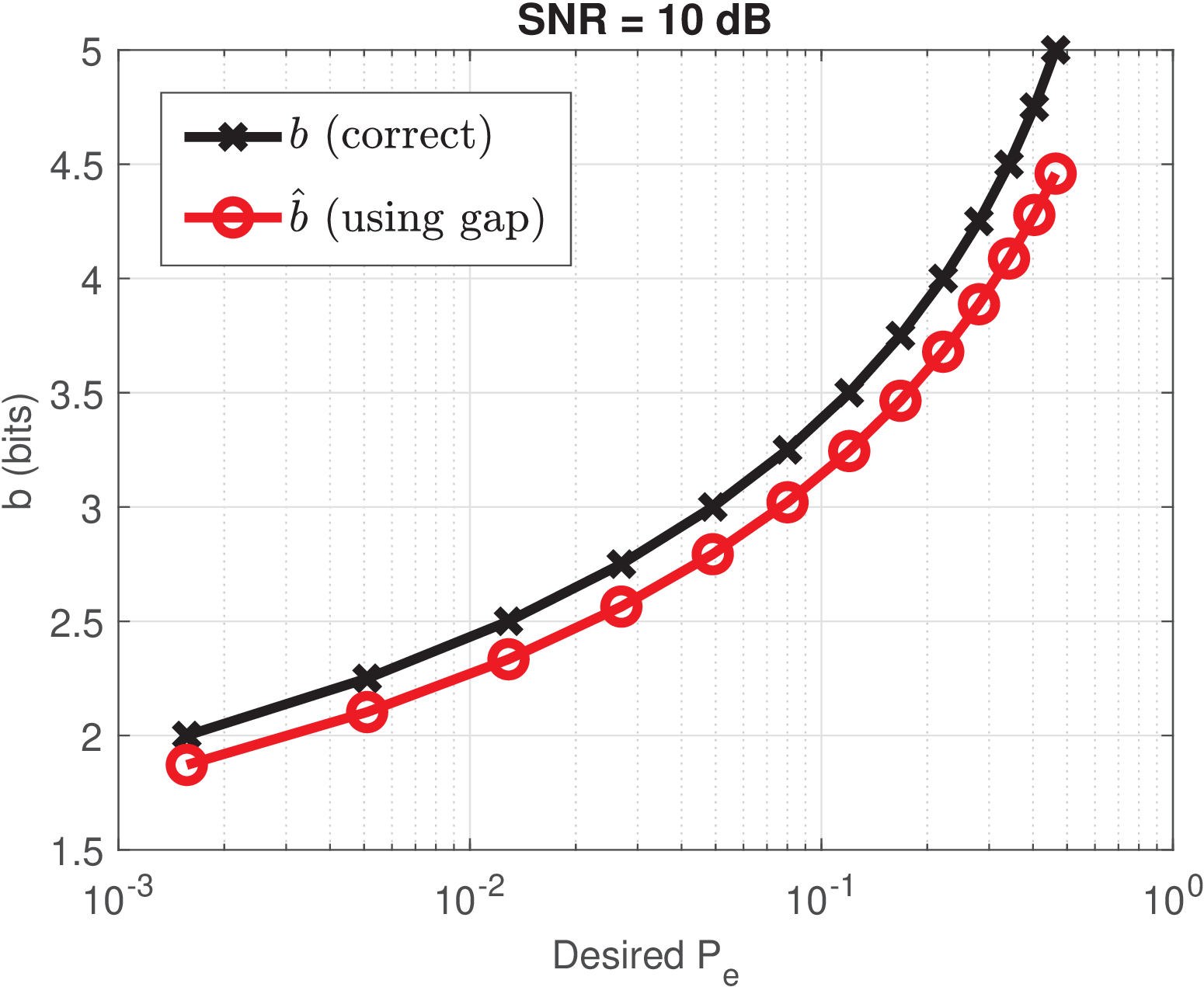
Figure 5.19 assumes that given $\mathrm{\text{SNR}}$ and $P_e$, the gap approximation is evaluated by comparing the number of bits.

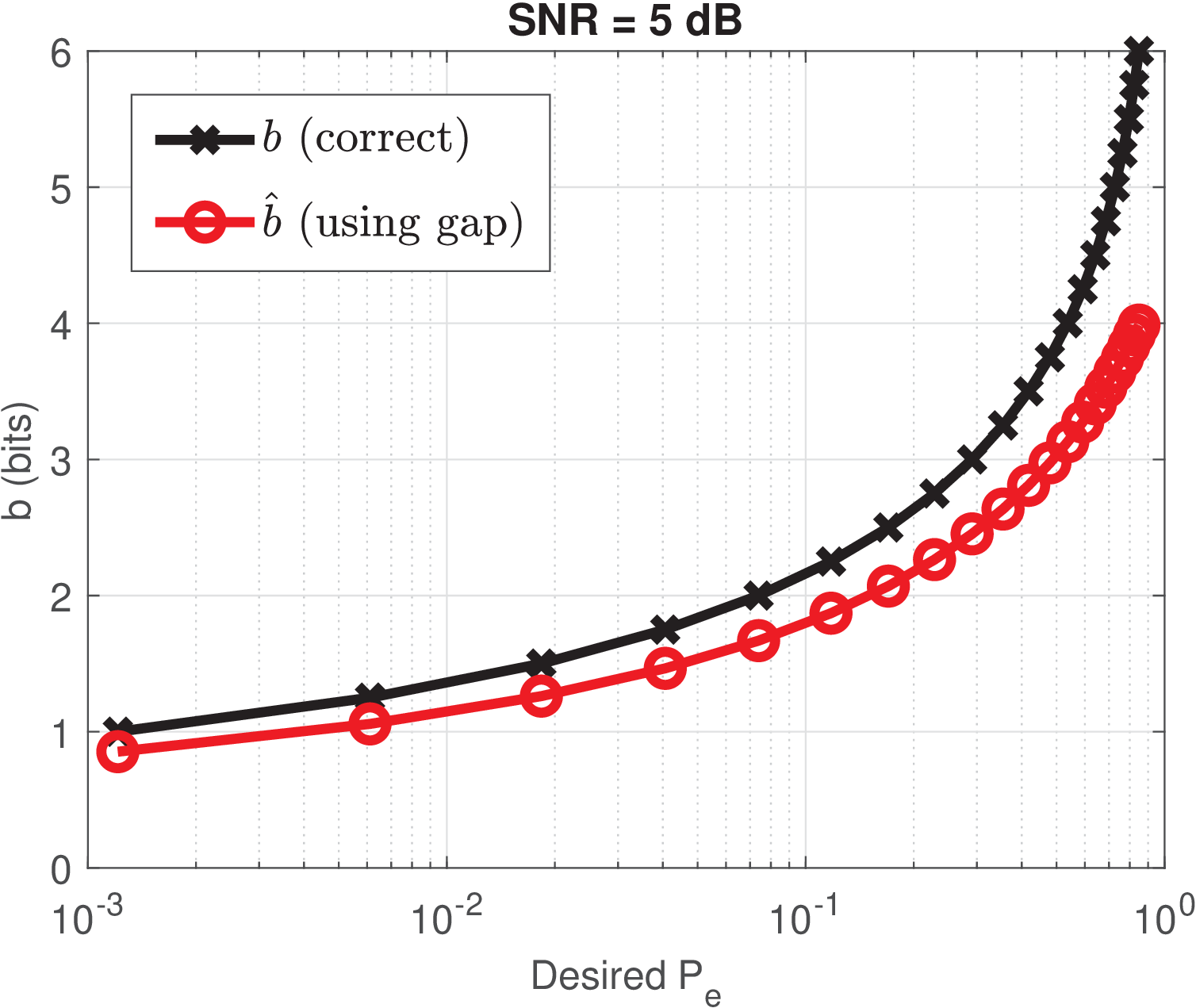
A similar procedure to Figure 5.19 was adopted to generate Figure 5.20 but, in this case, the SNR was decreased to $\mathrm{\text{SNR}}=\; 5$ dB. The impact on the accuracy of the gap approximation can be noticed when the SNR decreases, especially for high $P_e$.