Raised Cosine Shaping Pulses (Filters)

4.5 Raised Cosine Shaping Pulses (Filters)

When designing a communication system, the channel bandwidth is typically specified and the task is to design a transmit signal with a spectrum that fits within the bandwidth and can successfully convey information to the receiver. As discussed, the Nyquist criterion for zero ISI indicates reasonable values for the symbol rate and the desired property for the shaping pulse.

The most widely used set of functions that satisfy the Nyquist criterion, or Nyquist pulses, are the raised cosine pulses (or filters), given by:

p(t) = sinc (\frac{t}{T_{sym}}) [\frac{cos (\frac{rπt}{T_{sym}})}{1 − {(\frac{2rt}{T_{sym}})}^{2}}],

(4.28)

where $0 ≤ r ≤ 1$ is the roll-off factor, which controls the pulse bandwidth (more strictly, the transition band in frequency domain when interpreting $p(t)$ as the impulse response of a filter). Note that when $r = 0$ , Eq. (4.28) becomes the $sinc$ function.

Also note that Eq. (4.28) has singularities at $t = 0$ and $t = ± T_{sym} ∕(2r)$ . Using L’Hospital’s rule leads to $p_{sr} (t) |_{t=0} = 1$ and $p_{sr} (t) |_{t=± T_{sym} ∕(2r)} = \frac{π}{4} sinc (\frac{1}{2r})$ .

Recalling that the oversampling is $L = T_{sym} ∕ T_{s}$ and noting that $t$ is always normalized by $T_{sym}$ in Eq. (4.28), it is straightforward to rewrite Eq. (4.28) to obtain its discrete-time version. At the sampling instants $t = n T_{s}$ , one has $t∕ T_{sym} = (n T_{s})∕ T_{sym} = n∕L$ , which leads to

p[n] = sinc (\frac{n}{L}) [\frac{cos (\frac{rπn}{L})}{1 − {(\frac{2rn}{L})}^{2}}] .

(4.29)

When using a raised-cosine pulse in practice, the pulse needs to be truncated. For example, one may only consider the time interval from $− 5 T_{sym}$ to $5 T_{sym}$ ( $p(t)$ is assumed here to be symmetrical with respect to $t = 0$ ). After truncation, a delay is added to make the filter causal.

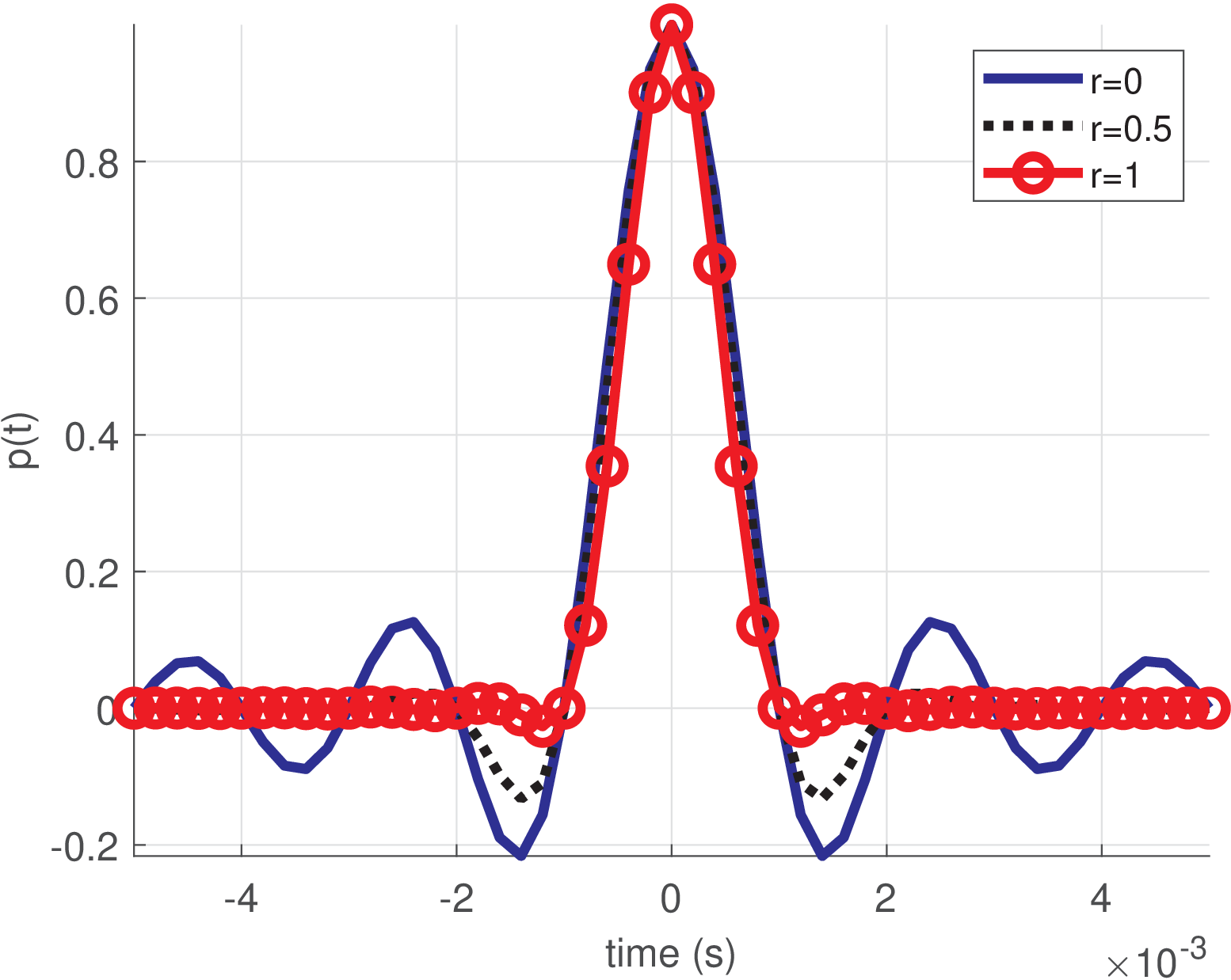
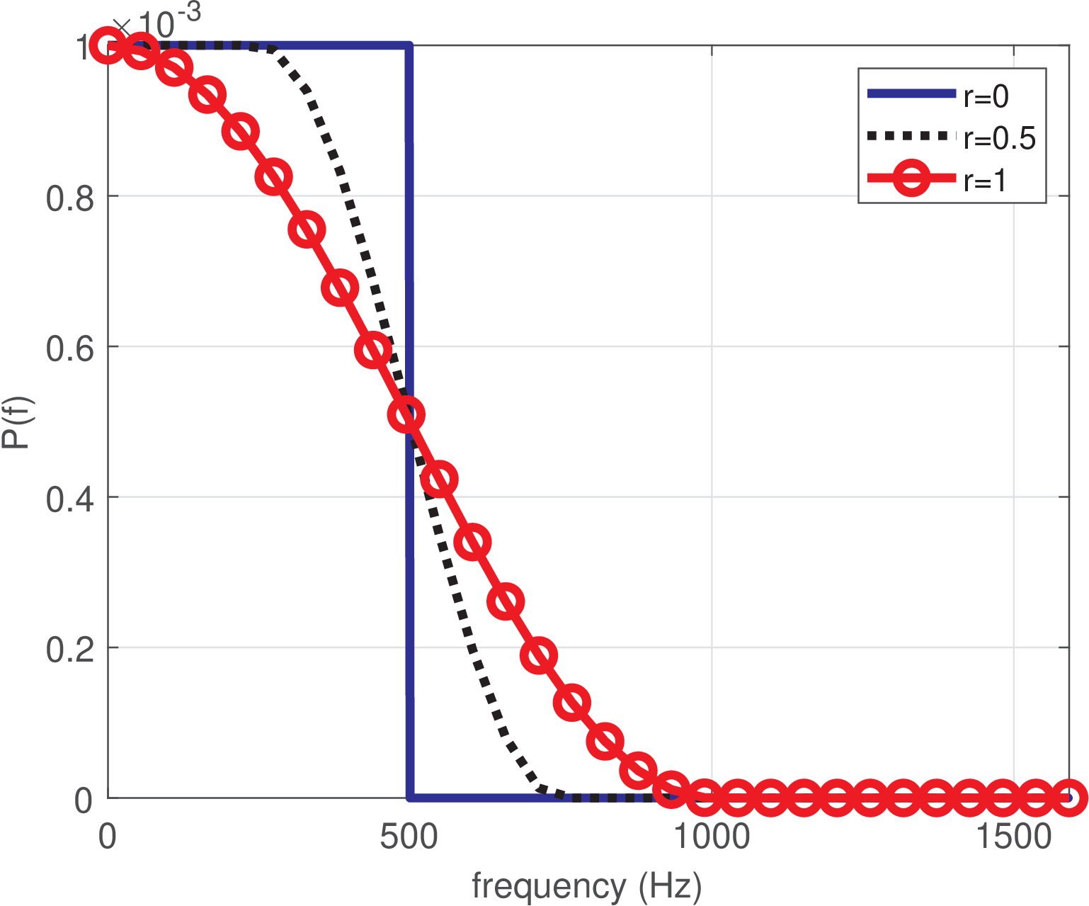
Figure 4.29: Raised cosines with $R_{sym} = 1000$ baud and roll-off $r = 0,0.5$ and 1.

Figure 4.29(a) shows raised cosines with $R_{sym} = 1000$ bauds and roll-off $r = 0,0.5$ and 1, while Figure 4.29(b) shows these pulses in the frequency domain. The spectrum of a raised cosine pulse is given by

P(ω) = {\begin{matrix} T_{sym}, & |ω|≤ \frac{π}{T_{sym}} (1 − r) \\ \frac{T_{sym}}{2} [1 − sin (\frac{T_{sym}}{2r} (|ω|− \frac{π}{T_{sym}}))], & \frac{π}{T_{sym}} (1 − r) ≤|ω| and \\ |ω|≤ \frac{π}{T_{sym}} (1 + r) \\ 0, & \frac{π}{T_{sym}} (1 + r) ≤|ω| \end{matrix}

(4.30)

Figure 4.30: Equivalent to Figure 4.22 with a raised cosine pulse with $r = 0.5$ .

Figure 4.31: Equivalent to Figure 4.23 with a raised cosine pulse with $r = 0.5$ .

Listing 4.6: MatlabOctaveCodeSnippets/snip_digi_comm_rcosine_timedomain.m

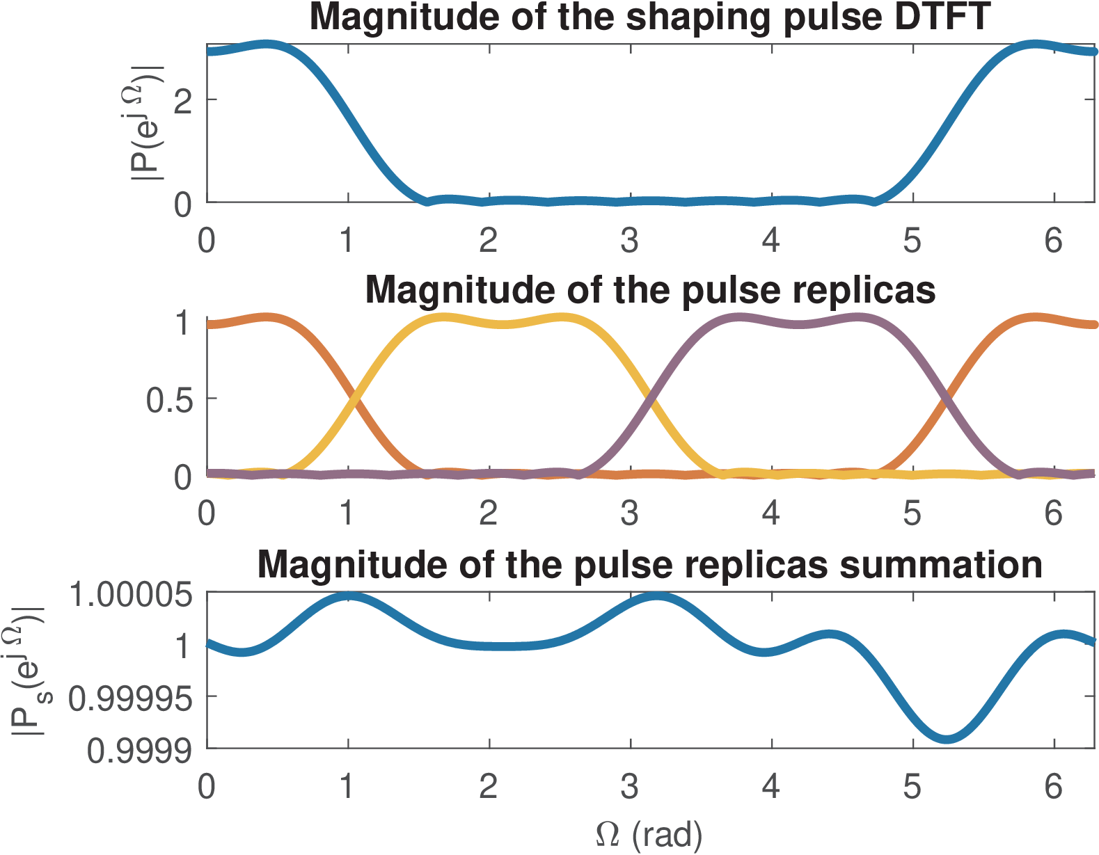
1L=3; %oversampling factor (samples per symbol) 
2r=0.5; %roll-off factor 
3Dsym=2; %group delay considering the number of input symbols at Rsym 
4p=ak_rcosine(1,L,'fir/normal',r,Dsym); %normal (not square-root) FIR 
5ak_plotNyquistPulse(p,L) %plot spectrum replicas in frequency domain 
6Ds=(length(p)-1)/2;%group delay considering output samples at Fs

Figure 4.30 and Figure 4.31 show graphs obtained with Listing 4.6. Application 4.2 discusses how to generate raised cosine filters in more details and it may be worth a peek. When using the rcosine function in Matlab (Octave misses it and here the companion ak_rcosine is assumed but the syntax is the same), a confusing aspect is that the fifth input parameter, the group delay, is accounted as the number of symbols (at $R_{sym}$ rate) not of samples (at $F_{s}$ rate). For example, in Listing 4.6 this delay $D_{sym}$ of 2 symbols, in combination with an oversampling of $L = 3$ , gives a filter with a delay (in samples) of $D_{s} = D_{sym} × L = 6$ and consequently the order of the filter is 12 (the filter has 13 taps or coefficients). Note that, in this case, $D_{s}$ was calculated assuming length(p) is an odd number.

In summary, the FIR raised cosine is symmetric and has a constant group delay in the passband. This delay can be accounted as $D_{sym}$ in number of symbols or $D_{s}$ in number of samples.

The roll-off can be written

r = (BW − {BW}_{min})∕ {BW}_{min},

where ${BW}_{min} = R_{sym} ∕2$ is the minimum bandwidth at a given symbol rate. Hence, the required bandwidth when using a raised cosine is

BW = {BW}_{min} (1 + r)

or, equivalently,

BW = \frac{R_{sym}}{2} (1 + r) (in Hz),

when $R_{sym}$ is in bauds.

Note that when dealing with raised cosines, $BW$ should not be understood as the 3-dB bandwidth, but the null-to-null bandwidth that includes passband and transition bands, from DC to the beginning of the stopband imposed by the first zero of the sinc. Eq. (4.30) describes the spectrum mathematically. Hence, in continuous-time, the passband ${BW}_{min}$ of a raised cosine is determined by $R_{sym}$ (or, equivalently, $1∕ T_{sym}$ ) because $R_{sym}$ determines the sinc of $p(t)$ with spectrum given by Eq. (A.54). The value of $r$ controls the cosine parcel and, together with $R_{sym}$ , determines the transition band with width $r {BW}_{min}$ .

In discrete-time signals, the parcel corresponding to the sinc in Eq. (4.29) has spectrum with bandwidth $π∕L$ rad as given by Eq. (A.54), such that

BW = \frac{π}{L} (1 + r) (in rad),

as indicated, for example, in Figure 4.32, where $BW = π∕3(1 + 1) ≈ 2.09$ rad.

While $R_{sym}$ and $r$ control $BW$ , the number of coefficients of the shaping pulse (or, equivalently, the order of this FIR filter) determines its attenuation in the stopband and group delay.

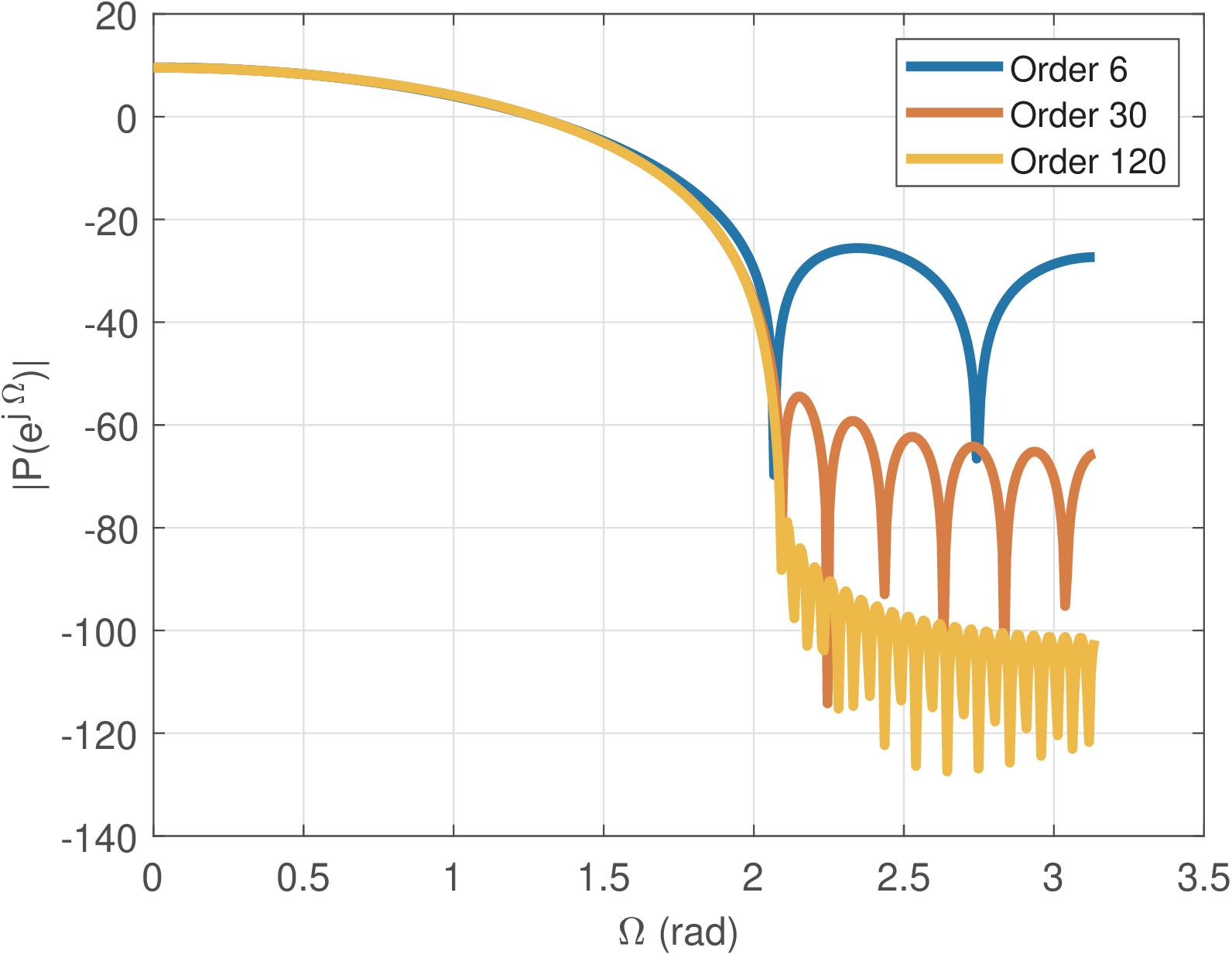
Figure 4.32: Comparison of raised cosine filters with $r = 1,L = 3$ and different orders.

Figure 4.32 compares raised cosine pulses with $r = 1,L = 3$ and different orders, obtained with the command p1=rcosine(1,L,[],r,N), where N=1,5 and 20. For example, in Figure 4.32, $L = 3$ and according to Eq. (A.54), the sinc parcel of the raised cosine imposes a ${BW}_{min}$ of $π∕3 ≈ 1.05$ rad. Because $r = 1$ , the cosine part of Eq. (4.29) creates a transition band of an extra 1.05 rad such that $BW ≈ 2$ rad.