3.9 Applications
Application 3.1. A simplified version of an ITU-T V.21 FSK-based modem. A very simple discrete-time example of FSK modulation is provided as Matlab/Octave code in the companion software (script fsk_synchronous.m in directory FSKSynchronous). The adopted parameters are the ones of the V.21 modem standardized by ITU-T. The task is to transmit an image and recover it after passing by a simulated channel.
The image was generated with script imageConversion.m and is a binary image, for simplicity. Figure 3.15 shows the image, which has white pixels corresponding to bit 1 and black pixels corresponding to bit 0. The bits 0 and 1 are represented by sinusoids with frequencies and , respectively.

The script implements two channels: the ideal (the received waveform is equal to the transmitted) and a noisy channel, which adds Gaussian noise with power 10 mW to the transmitted waveform.
Two different sets of frequencies were used. The first consisted of Hz, Hz, sampling frequency Hz and symbol rate bauds. In this case the basis functions are orthogonal and the number of samples per symbol is 80. The second set adopted Hz, Hz, Hz and bauds. In this latter case, the basis functions are not orthogonal. The number of samples per symbol is 32. This is compatible with the fact that binary FSK system typically do not use correlative demodulation and are based on simpler techniques that use filtering and the signal energy. Therefore, in many practical FSK implementations, orthogonality is not the issue.
Combining the two channel models with the two sets of frequencies led to Figure 3.16. The plots indicate that the noise was not strong enough to cause errors. The non-orthogonality of the basis functions cause a bias in the received coefficients, which is also not strong enough to provoke errors.
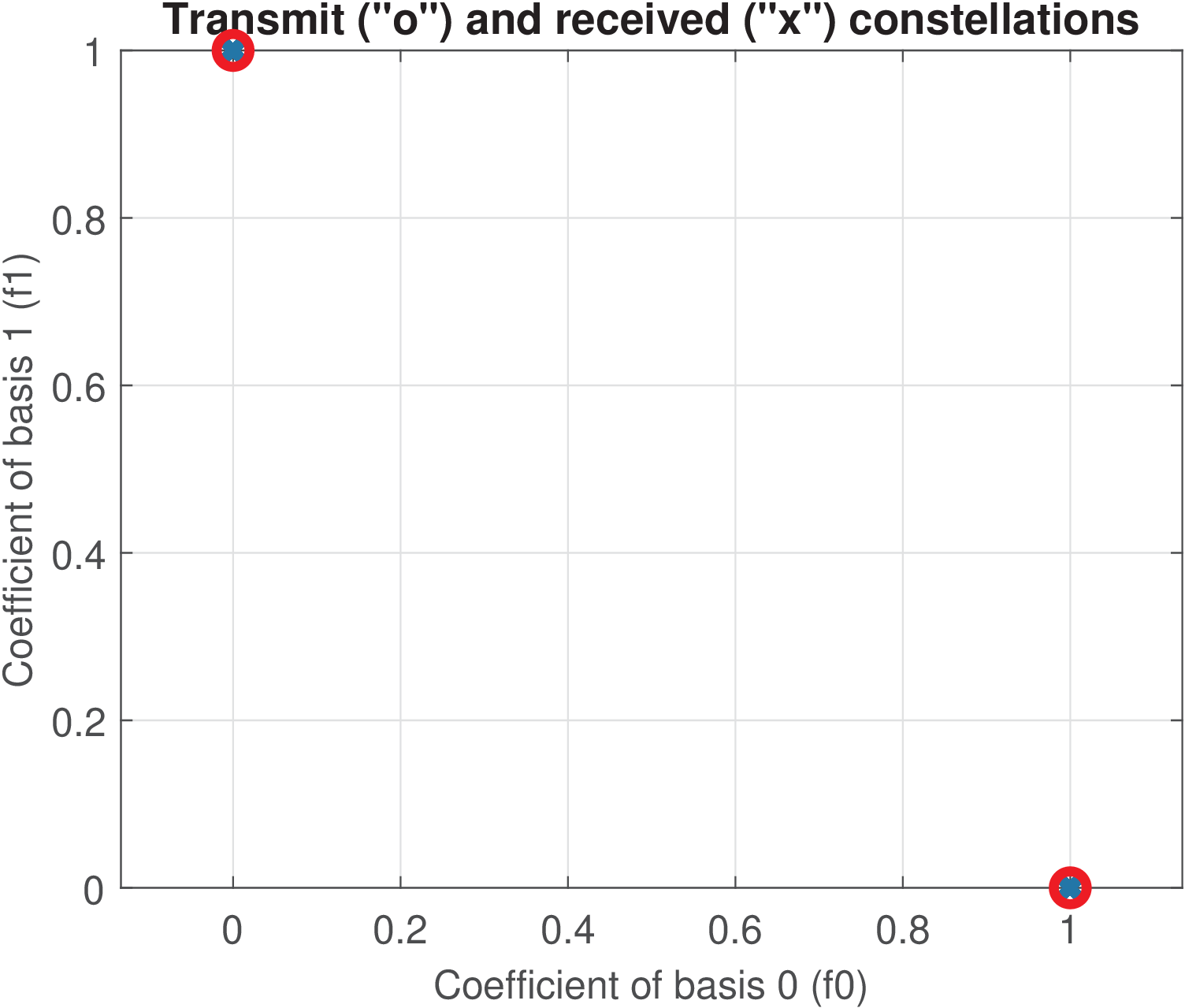
(a)
Ideal
channel
and
orthogonal
bases. |
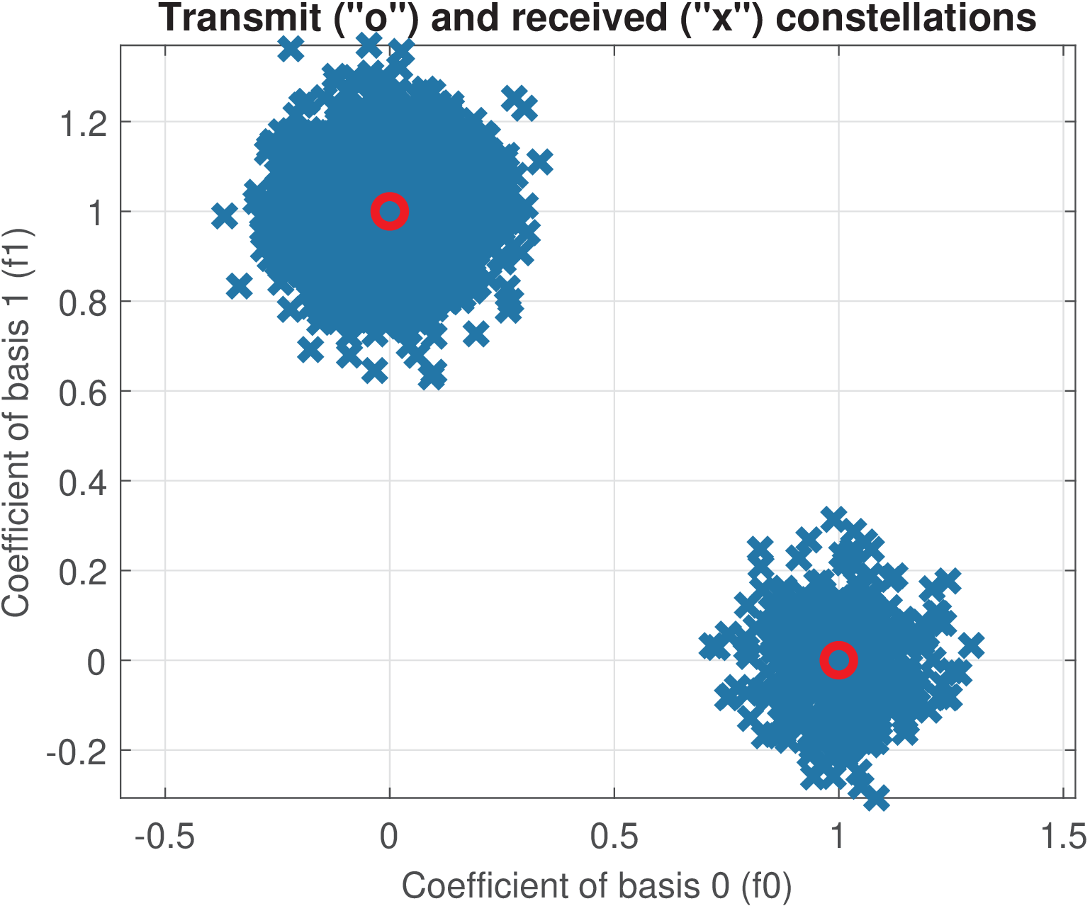
(b)
Noisy
channel
and
orthogonal
bases. |
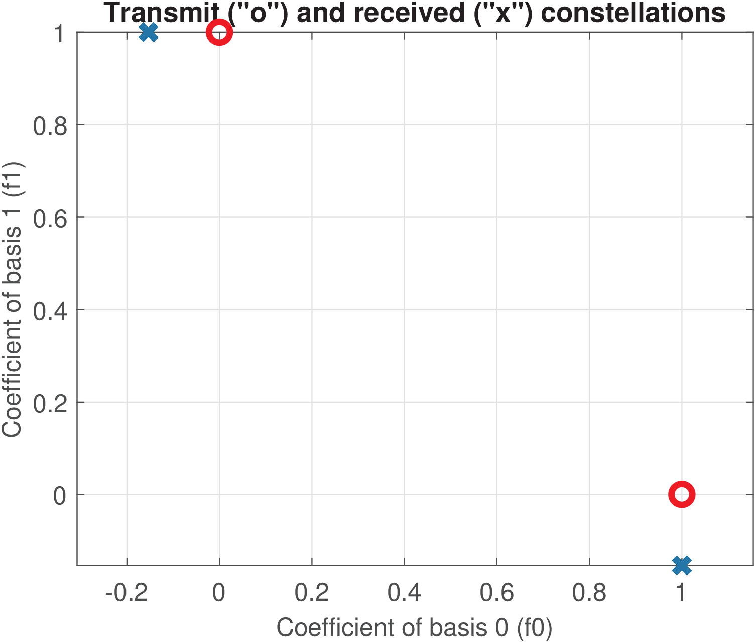
(c)
Ideal
channel
and
non-orthogonal
bases. |
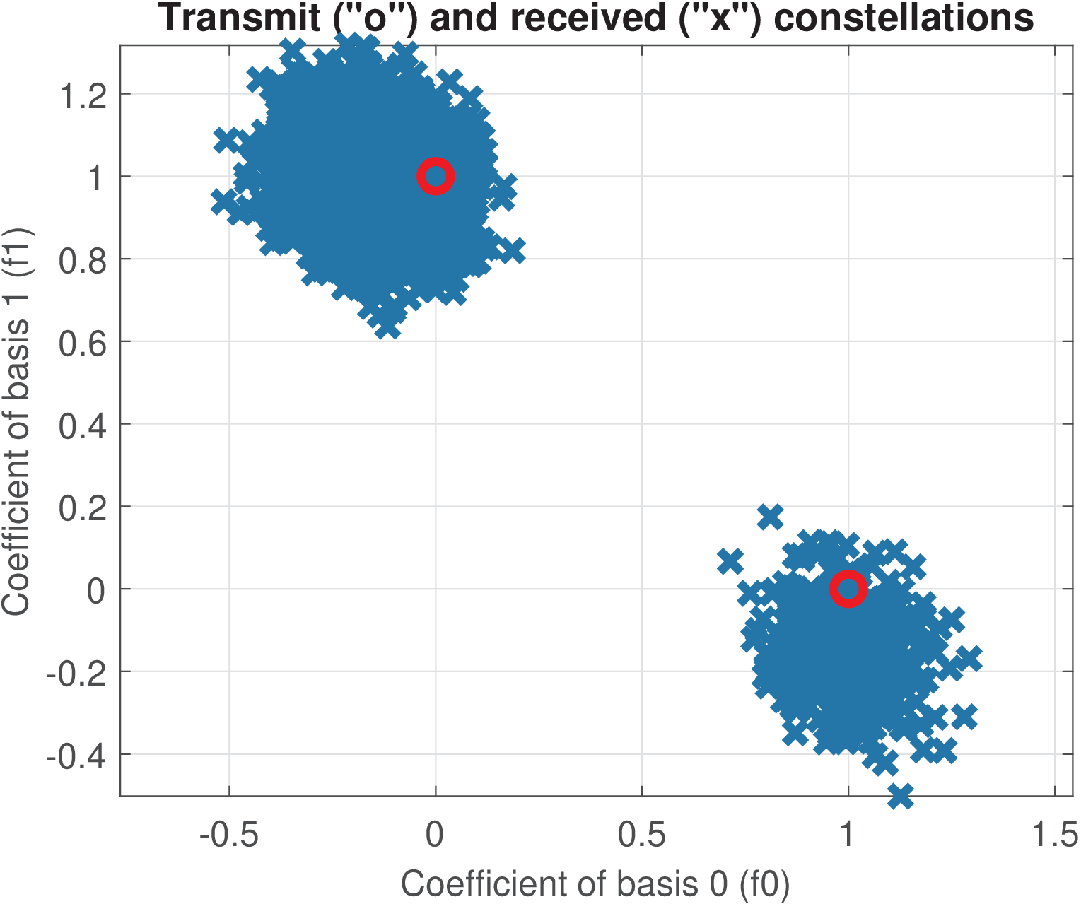
(d)
Noisy
channel
and
non-orthogonal
bases. |
It should be noted that, because the transmitted constellations are the same in all cases and the transform is unitary, all modulated waveforms corresponding to symbols have the same energy of 1 J. For the first set of frequencies, the signal power is 1/80 = 31.3 mW. For the second set of frequencies, the signal power is 1/32 = 12.5 mW. Given that the noise power is 10 mW in both cases, the signal to noise ratios are dB and , respectively. In this case, one could think that the noise impact would be more prominent for the first set of frequencies. However, Figure 3.16 indicates that, discarding the bias due to the non-orthogonality, the noise has a similar distribution around the transmitted symbols for both sets of frequencies. This is a consequence of the fact that in correlative demodulation, the important parameter is the symbol energy, not the waveform SNR. Intuitively, one can think that the energy was distributed among more samples in the first case, which decreased the power, but the receiver has more samples to take into account when making its decision via an inner product.
Application 3.2. Demodulation of the digitized complex envelope of a signal corresponding to multiplexed real-life AM stations. The experiment here is related to Application 1.2, but instead of the real-valued signal stored in am_real.wav, it uses a complex-valued signal stored in file am_usrp710.dat, which is available on the Web and must be downloaded (around 20 MB).4 This file stores a complex envelope obtained with a USRP software-defined radio platform.
The USRP was tuned to capture a radio frequency (RF) band centered at 710 kHz and the original signal was downsampled to create a complex-valued signal with approximately 11 seconds at kHz. The corresponding RF band of 256 kHz, from to kHz, was mapped to or, equivalently, kHz. For example, the three frequencies , 0 and 10 kHz of correspond to RF frequencies 700, 710 and 720 kHz, respectively. Figure 1.7 shows the PSD of with the abscissa showing the corresponding RF frequencies. The abscissa indicates the RF frequencies, but could show [-128, 128] kHz instead, with a RF carrier of 710 kHz.
As can be seen in Figure 1.7, because is complex, its PSD does not have Hermitian symmetry. Besides, each individual AM channel also does not have a spectrum with Hermitian symmetry with respect to its center frequency given that the channel impacted its lower and upper bands differently.
The script ak_showRadioTuner.m can be used to listen the AM stations represented in .
The script ak_convertAMComplexEnvelopeIntoRealValued.m was used to convert the signal in am_usrp710.dat into the real-valued signal stored in am_real.wav and detailed in Application 1.2.
Application 3.3. QAM simulation. The next paragraphs concerns the combined effects of a channel with band-limiting filtering and noise. The adopted approach is to work with a QAM system. The code is at directory Applications/QAMSynchronous and can be executed with different parameters.
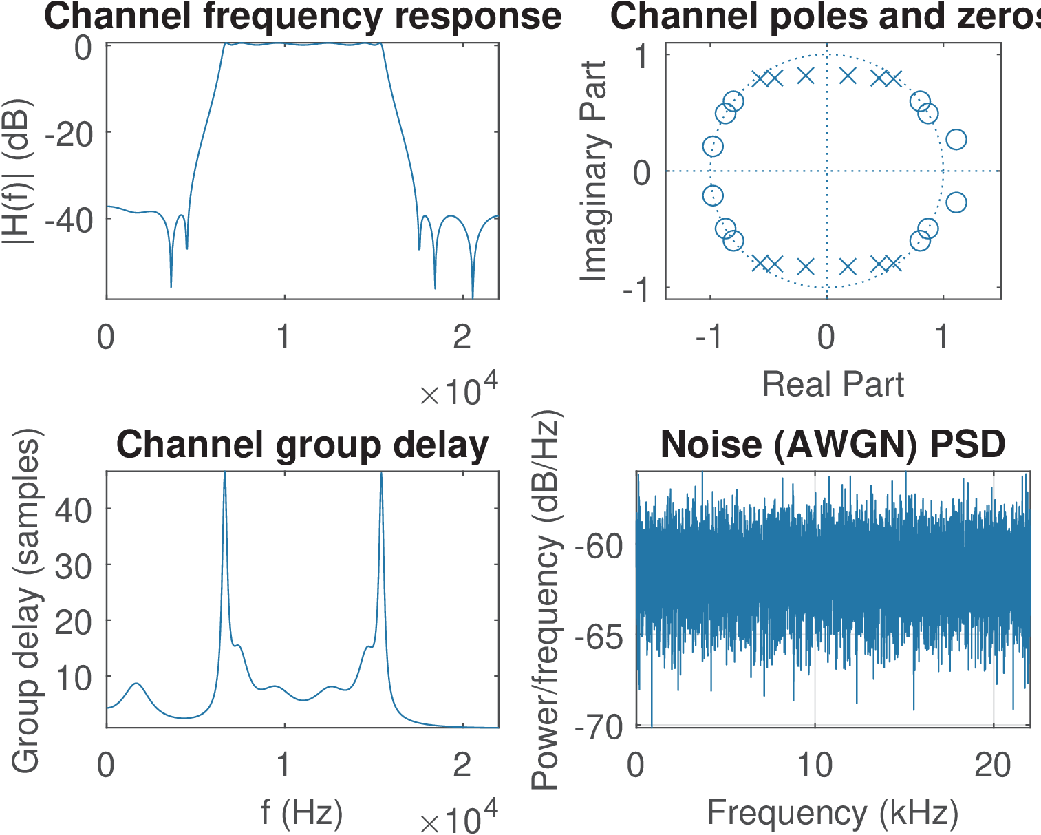
Figure 3.17 illustrates the simulated channel, which has a bandwidth of approximately 2 kHz, centered at Hz. There are zeros outside the unit circle, hence the channel is not minimum phase. The group delay is approximately 7 samples (equivalent to s) at the center frequency but has peaks closer to the cutoff frequencies. Hence, it is better to confine the transmit PSD within the frequency range that has an approximately constant group delay and gain.
The following example assumes kHz, dB, oversampling , carrier frequency = rad (equivalent to ), bauds, symbols and bps. Simulating with symbols led to an estimated BER=0. The average constellation energy is J, the energy of the shaping pulse is , the “theoretical” power of the upsampled signal is W, the power of the baseband complex envelope can be obtained via Eq. (E.101) and assuming the symbols are independent, such that W. The power of the transmitted signal is half of due to the upconversion. These “theoretical” values can be obtained with the commands in Listing 3.12 (but first, execute the initialization code dt_setGlobalConstants.m).
1Ec = mean(abs(const).^2)
2Eh = sum(htx.^2)
3Px = Ec/L
4powerTxComplexEnvelope = Px * Eh
5powerTxSignal = powerTxComplexEnvelope/2
The results of Listing 3.12 can be compared to the ones obtained via the simulation. The power of the signal at the receiver’s input depends on the transmitted signal bandwidth, which determines how the channel attenuates the transmitted signal. Assuming the transmitted signal has a narrow bandwidth, centered at the channel center frequency (which has a gain of 0 dB), the received power is approximately the transmitted power plus the WGN power. For example, using leads to a narrow PSD for the transmitted signal such that there is no significant channel attenuation. The received power is just slightly larger than the transmitted power. For an dB, the “theoretical” values are:
which corresponds to 0.0162 and 0.1787, respectively. The second command corresponds to Eq. (4.3) with the assumption that the noise samples are uncorrelated from the transmitted signal samples , such that . In this case their powers can be summed. The simulated values are and Watts, for the noise and received power, respectively. The AWGN PSD is noisePower/Fs W/Hz, which is a constant value (the noise is white) denoted as . In dB this PSD value is . Check at Figure 3.17 that the noise PSD is given by 10*log10(0.0166/10000) = -57.8 dB.
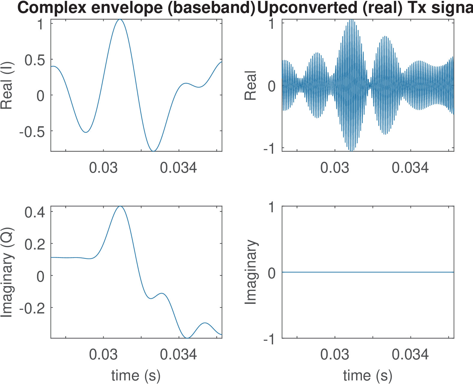
Figure 3.18 provides information about the transmitted signal in time domain. Note that the baseband signal is complex, while the signal transmitted over the channel is real. The shown time interval corresponds to 5 symbols (i. e., ). The in-phase component tends to have a larger amplitude than the quadrature component given that the constellation has symbols with larger real than imaginary part, as shown in Figure 3.19.
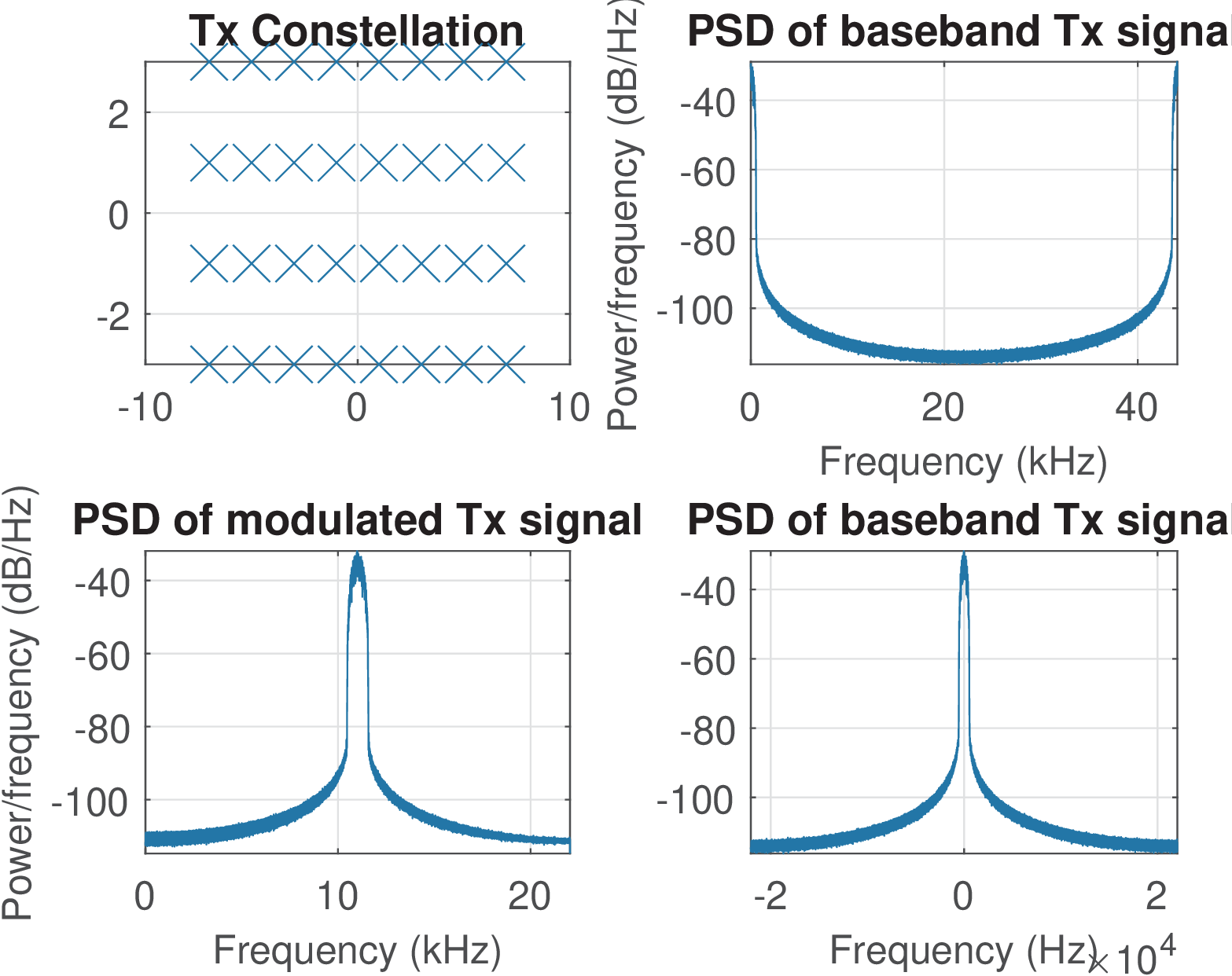
Figure 3.19 provides information about the transmitted signal in frequency domain. Two views of the PSD are provided for the baseband signal. Both used the pwelch command, which by default estimates the PSD using frequencies rad when the signal is real and Hermitian symmetry holds. When the signal is complex, the PSD is estimated in the range rad. When is informed, the PSD for complex-valued signals can be confusing because the abscissa is converted from to . Assuming the baseband complex envelope is yce, the two right-most plots of Figure 3.19 were obtained with the commands in Listing 3.13. It is important to get used to observing PSDs of complex-valued signals in Matlab/Octave and properly interpret alternatives to displaying the PSD over the range rad.
1subplot(222); pwelch(yce,[],[],[],Fs); %yce and Fs previously defined
2Pyce=pwelch(yce,[],[],[],Fs); %recalculate PSD, store result in Pyce
3f=linspace(-Fs/2,Fs/2,length(Pyce)); %create a frequency axis
4subplot(224); plot(f,fftshift(10*log10(Pyce))); %from -Fs/2 to Fs/2
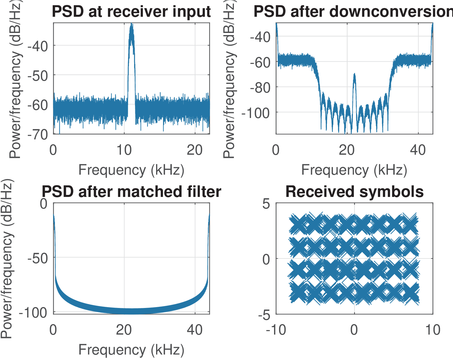
Figure 3.20 provides information about the received signal. The analytic signal is obtained with the aid of a Hilbert filter and downconverted to baseband. One important task is to estimate the best instant for starting sampling at the output of the matched filter. The code uses a global variable called delayInSamples to determine this instant. This variable gets updated by the average group delay at the band of interest after each filtering operation. For example, if a linear phase FIR with group delay equal to 4 samples is used, the variable is updated with delayInSamples=delayInSamples+4.
From Figure 3.20, the constellation at the receiver seems to suggest errors but running the code and zooming it, one can observe that the received symbols do not fall outside their correct (Voronoi) region.
The main script is dt_digital_transmission, which is listed below. Most parameters are specified at script dt_setGlobalConstants.
1%Example of digital transmission (part of application QamSynchronous)
2dt_setGlobalConstants %set global variables, script in companion code
3temp=rand(Nbits,1); %random numbers ~[0,1]
4txBitStream=temp>0.5; %bits (0 or 1) as a column vector
5s=ak_transmitter(txBitStream); %transmitter
6%choose channel:
7if useIdealChannel==1
8    r=s;
9else
10    r=dt_channel(s);
11end
12%rxBitStream=ak_receiver(r, phaseCorrection); %receiver
13rxBitStream=ak_receiver(r); %receiver
14%estimate BER (both vectors must have the same length)
15BER=ak_estimateBERFromBits(txBitStream, rxBitStream)
16baud = Fs/L
17rate_bps = baud*b
To practice, tune the parameters of the discussed QAM simulation to maximize the rate for a given BER. For example, decreasing the oversampling factor allows a larger at the expense of increased transmitted signal bandwidth.
Application 3.4. QAM over the sound board. Sound boards and Matlab/Octave allow to test many practical aspects of communication systems. Here, the QAM transmission system of Application 3.3 is modified to use the sound board and observe synchronization issues. The code is at directory Applications/QAMSynchronous.
A loopback cable connects the sound board DAC and ADC, as described in Application C.4. Then, the transmit QAM signal is sent to the DAC with the script ak_continuouslyTransmitQAM.m and recorded with the ADC using Audacity (or another sound recording software). The sound volume is adjusted to avoid having large amplitudes saturating the ADC and the recorded signal is saved as a WAV file. The script ak_offlineReceiveQAM.m implements the QAM receiver, reading the WAV file and processing it. This is an offline processing that is less complicated than implementing an online version. For example, a related challenge for an online implementation is to make Matlab/Octave process the signals using a given sampling frequency . This can be done with Playrec as in Application E.1 or the Java code of Application E.2, but only the offline version is discussed here.
Even in this case of a simple loopback cable, an important issue when moving from a simulated channel to a real (physical) one is to deal with synchronization. In the simulation of Application 3.3, the global variable delayInSamples is updated by the transmitter and channel, such that the receiver knows when to start downsampling the waverform to extract the symbols. In other words, with a simulated channel, it is relatively easy to avoid the need for symbol timing recovery strategies. For the current application, the timing was solved as follows: the transmit bitstream was fragmented in frames and a preamble (known to both transmitter and receiver) was pre-appended to each frame. This preamble is an M-sequence (see Section 4.9.1), which is designed to have a peak as its autocorrelation. Thus, a cross-correlation between the received signal and the preamble helps to identify the sample index corresponding to the preamble start within the received signal.
The preamble can also be used to equalize the channel. In the simple receiver implementation of ak_offlineReceiveQAM.m, because the transmit PSD is relatively narrowband, it was assumed that the channel modifies the transmitted symbols by a single complex value, given by , where is the carrier frequency (in this case, kHz). In other words, the preamble is composed by values (that are in M-sequences) and the received symbols are . Hence, the estimated adjustment when the preamble is composed by samples is
|
| (3.18) |
which is implemented in ak_offlineReceiveQAM.m with the line:
This corresponds to an equalizer with a single value or tap. This simple equalization is performed by , i. e., simply normalize the original received symbols by the complex value .
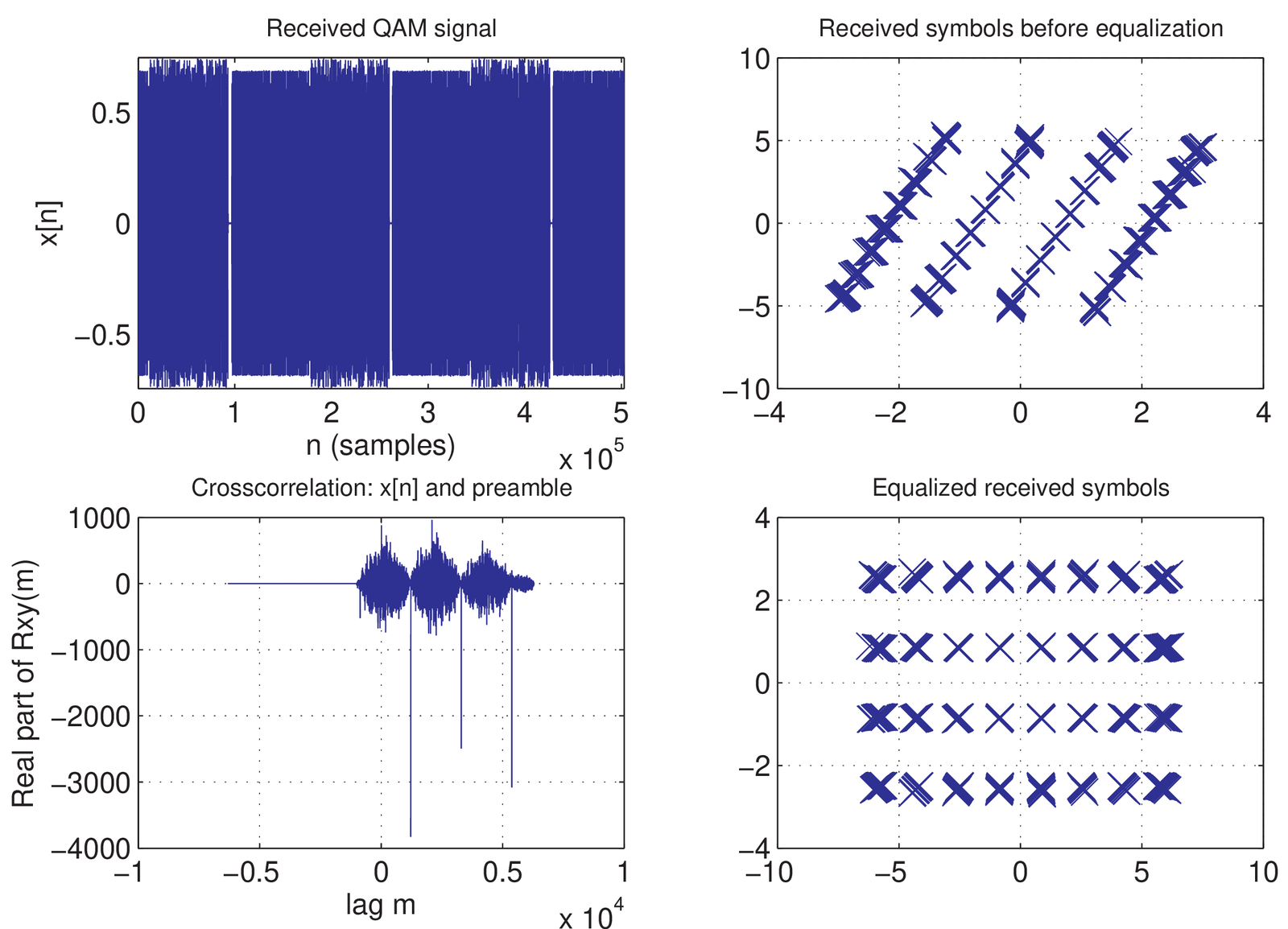
Figure 3.21 shows some results of the demodulation process. The synchronization is performed via cross-correlation and its peaks indicate the preamble presence. The described equalization procedure is capable of correcting the received symbols as illustrated by the equalized constellation. The effect of equalization is a rotation and scaling of the original constellation.
An interesting aspect of using a M-sequence preamble is that its uncorrelated values have a corresponding white frequency spectrum. Directly sending these samples to the DAC is not recommended because the channel has a limited bandwidth and the white spectrum would not conform to this restriction. Therefore, the preamble is upsampled and filtered by the shaping pulse in the same way as the transmit symbols. At the receiver, the waveform sampled at can be downsampled to the baud rate and the cross-correlation calculated between the preamble and a version of the received signal at the baud rate .5 It remains to determine the first sample to start the downsampling operation. In ak_offlineReceiveQAM.m this sample is obtained by a brute force approach, which tries all possibilities from 1 to the oversampling factor .
To estimate the BER, the transmitted information symbols must be known at the receiver. To simplify the BER estimation procedure, the same frame is repeatedly transmitted by ak_continuouslyTransmitQAM.m, which corresponds to sending the same bits in all frames. The transmitted bits are stored in the global variable txBitStream, which is made available to the receiver. The reader is invited to vary system parameters, for example, to maximize the bit rate and also implement a more sophisticated equalization procedure.