QAM Demodulation Using Complex-Valued Signals

3.5 QAM Demodulation Using Complex-Valued Signals

This section discusses QAM demodulation, i. e., the process of recovering the symbols embedded in the received waveform. The process can be organized into two tasks: 1) recovering the complex-valued symbols, i. e., an eventually noisy version of the complex envelope, and then 2) making decisions by finding the nearest-neighbor constellation point to each received QAM symbol. The second task is briefly discussed in the next paragraphs, assuming square QAM constellations.

3.5.1 PAM-based detector scheme for square QAM

Note that some “demodulation” functions in Matlab/Octave simply perform the decision or detection process. Here, sticking with this nomenclature, a function called ak_qamdemod.m is described.

The implementation of the decision stage is simplified if a square QAM (SQ QAM) constellation is adopted, where the number $b$ of bits in an even integer. As suggested by Figure 2.24, the SQ QAM constellation is the Cartesian product of two identical PAM constellations with $2^{b ∕ 2} = \sqrt{M}$ symbols each. Listing 3.4 illustrates the demodulation for this specific constellation. The case where $b$ is an odd number is not considered at this moment.

Listing 3.4: MatlabOctaveFunctions/ak_qamdemod.m

1function [symbolIndex, x_hat]=ak_qamdemod(x,M) 
2% function [symbolIndex, x_hat]=ak_qamdemod(x,M) 
3%It is restricted to "square" QAM constellations. It does 
4%not support "cross" constellations. 
5%Inputs: x has the QAM values and M the number of symbols 
6%Outputs: symbolIndex has the indices from 0 to M-1 
7%         x_hat contains the nearest symbol(s) 
8b=log2(M); %number of bits 
9b_i = ceil(b/2); %number of bits for in-phase component 
10b_q = b-b_i; %remaining bits are for quadrature component 
11M_i = 2^b_i; %number of symbols for in-phase component 
12M_q = 2^b_q; %number of symbols for quadrature component 
13ndx_i=ak_pamdemod(real(x),M_i); %PAM on in-phase 
14ndx_q=ak_pamdemod(imag(x),M_q); %PAM on quadrature 
15symbolIndex = ndx_i*M_q + ndx_q; %get QAM index 
16if nargout > 1 %calculate only if necessary 
17    const=ak_qamSquareConstellation(M); %QAM const. 
18    x_hat=const(symbolIndex+1);%add 1 to indices 
19end

The decision process is just one among other used for demodulation. The next paragraphs discuss distinct ways for estimating the complex envelope, which is a process that precedes the decision in many demodulation schemes.

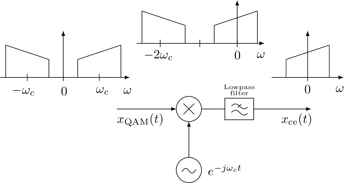
3.5.2 QAM demodulation of complex-valued signals with lowpass filter

As in the QAM generation stage, using complex-valued signals can help mathematically describing and implementing QAM demodulation.

When complex-valued signals are used, Figure 3.7 depicts an alternative for QAM demodulation. This demodulation used a lowpass filter and another alternative that will be discussed is to use a phase splitter, which incorporates a Hilbert filter.

Figure 3.7: QAM demodulation using lowpass filter that operates on complex-valued signals.

Hence, as an example of an alternative to accomplish QAM demodulation, Listing 3.5 illustrates how to recover the QAM symbols and leads to the same results as Listing 3.2. Note that the first lines of Listing 3.5 are not listed but coincide with Listing 3.3, which is used to obtain the transmitted QAM signal z.

Listing 3.5: MatlabOctaveBookExamples/ex_qam_demodulation_lowpass.m

17r = z;  %ideal channel: no noise (z already defined). Run QAM demod.: 
18n=0:length(r)-1; %integer indices that represent time evolution 
19wc=pi/2; %carrier frequency in radians 
20carrier=2*exp(-1j*wc*n); %generate complex carrier. Note factor = 2 
21rbb=r.*carrier; %shift one QAM replica to the baseband 
22b=fir1(length(p)-1,0.5); %FIR with same order of the shaping filter 
23ybb=conv(b,rbb); %filter out replica at twice the carrier frequency 
24ybb(1:floor(length(p)/2)+floor(length(b)/2))=[];%discard group delays 
25ys=ybb(1:L:L*S); %sample S symbols, at baud rate 
26symbolIndicesRx=ak_qamdemod(ys,M); %QAM demodulation 
27SER=ak_calculateSymbolErrorRate(symbolIndicesRx,ind)

Listing 3.6 provides code to show the original constellation and the received symbols.

Listing 3.6: MatlabOctaveCodeSnippets/snip_digi_comm_QAM_result.m

1%Plot constellation (ys has been previously defined): 
2plot(real(ys),imag(ys),'x','markersize',20); %received 
3hold on, plot(real(qamSymbols),imag(qamSymbols),'or'); %transmitted 
4axis equal; axis([-4 4 -4 4]); %force axis to have same lengths 
5title('Transmitted (o) and received (x) constellations'); 
6xlabel('Real part of QAM symbol m_i'); 
7ylabel('Imaginary part of QAM symbol m_q');

Figure 3.7 assumed continuous-time signals, but discrete-time processing can be used as well. For example, a single (and relatively fast) ADC can be used to digitize the passband QAM signal and the frequency downconversion and filtering performed in the digital domain.

3.5.3 Advanced: QAM demodulation of complex-valued signals via phase splitter

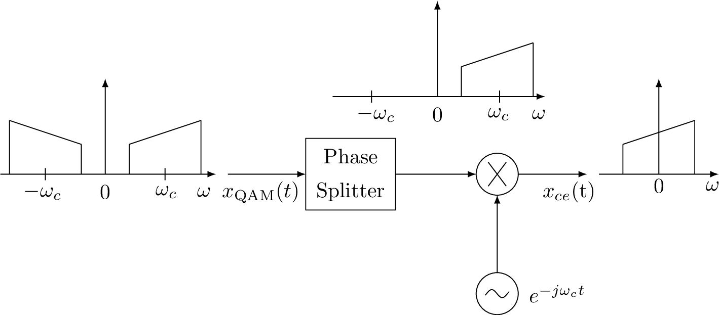
Now, the option of using a phase splitter via a Hilbert transform in QAM demodulation is discussed. Complementing the example provided by Figure 3.6, Figure 3.8 illustrates two stages in QAM demodulation: obtaining the analytic signal and downconversion. This first stage will be described in the sequel.

Figure 3.8: QAM demodulation using complex-valued signals: the analytic signal (middle plot) is downconverted to obtain the complex envelope (bottom). Only $X_{QAM} (f)$ presents Hermitian symmetry.

Using a unit step function $u (f) = 0.5 (1 + sgn (f))$ in frequency domain ( $sgn (\cdot)$ is the sign function) allows to obtain

u (f) X_{QAM} (f),

which eliminates the negative frequencies of the passband spectrum $X_{QAM} (f)$ . The goal is to obtain an analytic signal $x_{+} (t)$ to represent the passband signal $x_{QAM} (t)$ . An analytic signal has a spectrum that is zero for $f \leq 0$ . The inverse Fourier transform of $u (f)$ is

F^{- 1} {u (f)} = \frac{δ (t)}{2} + \frac{j}{2 πt} = \frac{1}{2} (δ (t) + j \frac{1}{πt})

where the factor $1 ∕ 2$ will be compensated by multiplying $u (f)$ by 2 (note in Figure 3.8 the multiplication by 2 when generating the analytic signal, which also shows up in Figure 3.6). Therefore, for convenience, the analytical signal is defined in frequency domain as

X_{+} (f) = 2 u (f) X_{QAM} (f) .

(3.8)

Interpreting the analytical signal in time domain leads to

\begin{align} x_{+} (t) & = F^{- 1} {X_{+} (f)} = 2 F^{- 1} {u (f) X_{QAM} (f)} = 2 F^{- 1} {u (f)} * x_{QAM} (t) \\ = x_{QAM} (t) + j (x_{QAM} (t) * \frac{1}{πt}) . & (3.9) \end{align}

At this point, it is helpful to note that

\bar{h} (t) = {\begin{matrix} \frac{1}{πt} & , t \neq 0 \end{matrix}

is the impulse response of a Hilbert filter and the Hilbert transform $\overset{ˇ}{x} (t)$ of a signal $x (t)$ is

\overset{ˇ}{x} (t) = x (t) * \bar{h} (t) = \int_{- \infty}^{\infty} \frac{x (u)}{π (t - u)} du .

Hence, one can obtain the analytic signal by means of a Hilbert transform as follows:

x_{+} (t) = x_{QAM} (t) * (δ (t) + j \frac{1}{πt}) = x_{QAM} (t) + j \overset{ˇ}{x} (t),

where $\overset{ˇ}{x} (t)$ in this case is the Hilbert transform of $x_{QAM} (t)$ . Note that the real part of $x_{+} (t)$ is the input signal $x_{QAM} (t)$ itself and the imaginary part is $\overset{ˇ}{x} (t)$ . A system that obtains the analytic signal $x_{+} (t)$ from a real input signal is called phase splitter. Figure 3.9 illustrates a phase splitter operating in continuous-time signals. It can also be used in discrete-time, for example, on a digitized passband QAM signal such that only one high-frequency ADC is used, instead of a dual ADC to digitize the I/Q components.

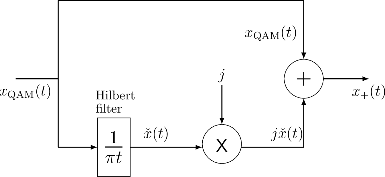
Figure 3.9: Phase splitter as used in QAM demodulation.

After the phase splitter of Figure 3.9, the QAM complex envelope can be obtained by frequency downconverting the resulting analytic signal, as depicted in Figure 3.10.

Figure 3.10: QAM demodulation using a Hilbert filter incorporated to a phase splitter.

While the Fourier transform of the phase splitter is $2 u (ω)$ , the transform of the Hilbert filter denoted by its impulse response $\bar{h} (t)$ is $\bar{H} (ω) = - j sgn (ω)$ . The top and bottom branches that compose the phase splitter of Figure 3.9 have Fourier transforms equal to 1 (top branch) and $j \times \bar{H} (ω) = sgn (ω)$ , such that their sum leads to $2 u (ω)$ .

Observing the role played by the Hilbert transform, $| \bar{H} (ω) | = 1, ω \neq 0$ and it does not alter the magnitude of the input $x (t)$ unless $X (0) \neq 0$ , which does not occur for passband signals. Hence, the Hilbert transform changes the signal phase by adding $- π ∕ 2$ rad to components at positive frequencies and $π ∕ 2$ to components at negative frequencies.

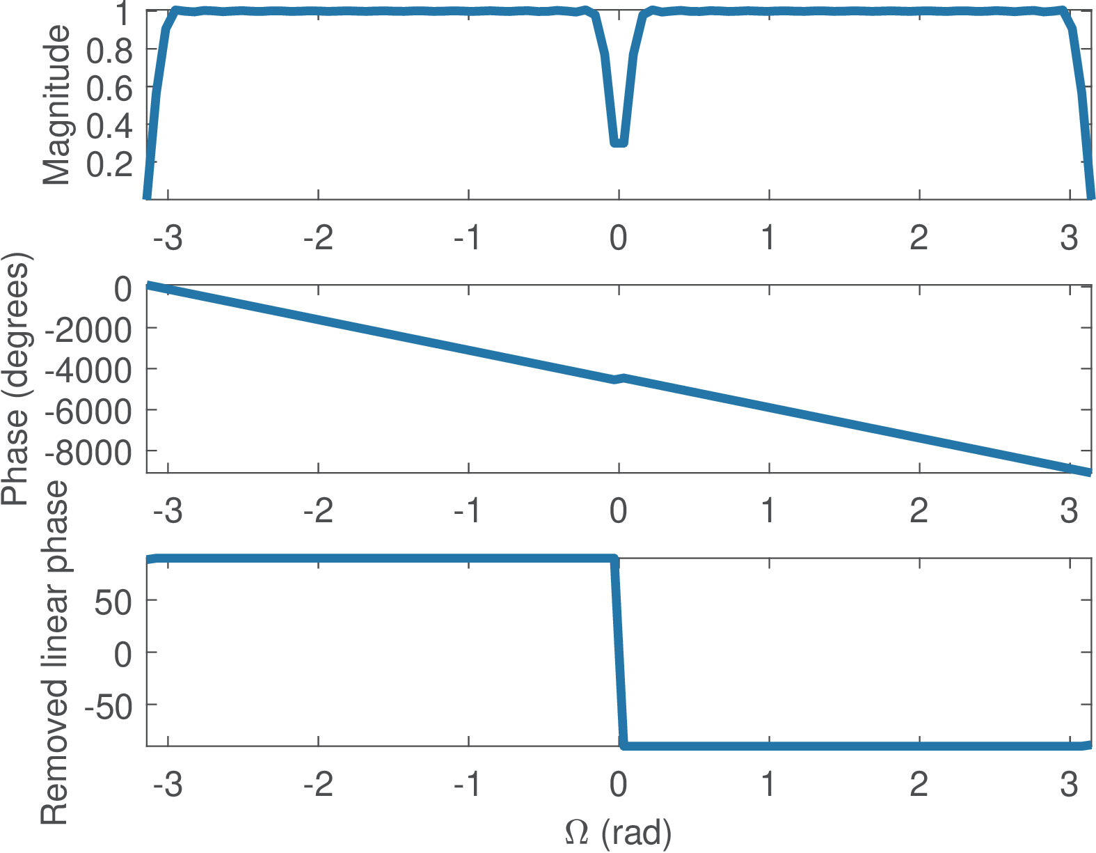
Figure 3.11: Magnitude (top) and phase (middle) of a 52-th order FIR Hilbert filter. The bottom plot is obtained by removing the linear phase factor.

Figure 3.11 depicts the frequency response of a Hilbert filter² obtained with Listing 3.7.

Listing 3.7: MatlabOnly/snip_digi_comm_hilbert_filter_design.m

1N = 52;           % Filter order 
2F = [0.05 0.95];  % Frequency Vector 
3A = [1 1];        % Amplitude Vector 
4W = 1;            % Weight Vector 
5b  = firls(N, F, A, W, 'hilbert'); %design Hilbert filter

Note that any causal FIR filter will have a linear phase that can hide the effect of a Hilbert transformer on the input signal’s phase (the $\pm π ∕ 2$ shift). The bottom plot in Figure 3.11 was obtained with Listing 3.8, where N/2=26 in this case.

Listing 3.8: MatlabOctaveCodeSnippets/snip_digi_comm_hilbert_filter_analysis.m

1w=linspace(-pi,pi,100); %frequency in rad 
2H=freqz(b,1,w); %calculate frequency response (b has been defined) 
3H2=H.*exp(j*(N/2)*w); %compensate linear phase 
4plot(w,angle(H2)/pi*180); %convert to degrees

When using filters, the transients need to be taken into account. Listing 3.9 illustrates the use of a causal Hilbert filter to recover the complex envelope.

Listing 3.9: MatlabOctaveBookExamples/ex_qam_demodulation_hilbert.m

17r = z;  %ideal channel, no noise, unlimited band (z was defined) 
18%run the demodulation using complex signals 
19%First design a Hilbert filter (or transformer) 
20N = length(p)-1;          % Order 
21F = [0.05 0.95];  % Frequency Vector 
22A = [1 1];        % Amplitude Vector 
23W = 1;            % Weight Vector 
24b  = firls(N, F, A, W, 'hilbert'); 
25yhilbert = conv(b,r); %Hilbert transform 
26yhilbert(1:floor(length(b)/2))=[]; %take out transient 
27ya = r + j*yhilbert(1:length(r)); %analytic signal 
28ybb = ya .* exp(-j*pi/2*n); %downconversion 
29ybb(1:floor(length(p)/2))=[]; %take out transient 
30firstSample = 1; %first sample to start getting symbols 
31ys=ybb(firstSample:L:L*S); %sample S symbols, baud rate 
32symbolIndicesRx=ak_qamdemod(ys,M); %QAM demodulation 
33SER=ak_calculateSymbolErrorRate(symbolIndicesRx,ind)

An alternative to using a causal filter is the hilbert function, which outputs the analytic signal and instead of a FIR filter uses FFT. Listing 3.10 illustrates the use of hilbert.

Listing 3.10: MatlabOctaveBookExamples/ex_qam_demodulation_complex.m

17r = z;  %ideal channel: no noise, unlimited band (z was defined) 
18%run the demodulation using complex signals 
19ya = hilbert(r); %get analytic signal 
20ybb = ya .* exp(-j*pi/2*n); %downconversion 
21ybb(1:floor(length(p)/2))=[]; %take out transient 
22firstSample = 1; %first sample to start getting symbols 
23ys=ybb(firstSample:L:L*S); %sample S symbols, baud rate 
24symbolIndicesRx=ak_qamdemod(ys,M); %QAM demodulation 
25SER=ak_calculateSymbolErrorRate(symbolIndicesRx,ind)

It should be noted that the hilbert function used in Listing 3.10 does not implement the Hilbert transform, but the complete phase splitter.

The following simple example aims at providing insight on recovering a signal after its components corresponding to negative frequencies were eliminated.

Example 3.1. Recovering a real-valued signal using only the values of its Fourier transform corresponding to positive frequencies. As an exercise and assuming discrete time, Listing 3.11 illustrates how to recover an arbitrary signal (representing $x_{QAM} [n]$ ) from the values $X_{+} [k]$ corresponding to positive frequencies of its FFT.

Listing 3.11: MatlabOctaveCodeSnippets/snip_digi_comm_ifft_qam_recover.m

1x=[1 2 3 4 5 6] %define an arbitrary test vector 
2X=fft(x); N=length(x); %calculate FFT and its length 
3Xu=[X(1) 2*X(2:(N/2)) X((N/2)+1)]; %Xu = 2 u(f) X(f) 
4x2 = real(ifft(Xu,N)) %use ifft zero-padding. find x2=x

Note in Listing 3.11 that the DC and Nyquist frequencies are not scaled by 2. $□$

² The Octave’s version of firls does not support the ’hilbert’ option.