QAM Represented with Real-Valued Signals

3.3 QAM Represented with Real-Valued Signals

The QAM signal is obtained by simultaneously using a cosine of frequency $f_{c}$ to upconvert a PAM and a sine of the same frequency $f_{c}$ to upconvert another PAM. In spite of these two passband PAM being superimposed (overlapping) in frequency, they can be individually recovered at the receiver. The details of QAM generation are described in the sequel.

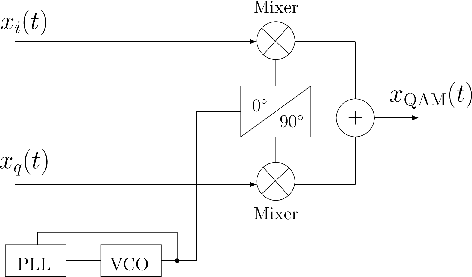
Using the same method of PAM generation from a single bitstream, one can create two PAM signals by splitting the original bitstream with rate $2 R$ into two, with rate $R$ each. Assuming continuous-time signals, these bitstreams are represented by PAM signals $x_{i} (t)$ and $x_{q} (t)$ , which are then multiplied by a cosine and sine, respectively, to create the QAM signal

x_{QAM} (t) = x_{i} (t) cos (ω_{c} t) + x_{q} (t) sin (ω_{c} t) .

(3.2)

Assuming the cosine as a reference, the sine is obtained by delaying it of 90 degrees, i. e., using the fact that $sin (𝜃) = cos (𝜃 - π ∕ 2)$ . Hence, $x_{i} (t)$ and $x_{q} (t)$ are called the in-phase (I) and quadrature (Q) components of a QAM signal, respectively. Figure 3.3 illustrates a possible QAM generation procedure.

Figure 3.3: QAM modulation where the PLL and VCO generate the carrier for the I component and, from this signal, the 90 degrees phase shifter creates the carrier for the Q component.

Trigonometry gives a hint on how the two PAM signals that compose a QAM signal can be recovered at the receiver. Multiplying $x_{QAM} (t)$ of Eq. (3.6) by $cos (ω_{c} t)$ and filtering, allows to recover $x_{i} (t)$ , while multiplying $x_{QAM} (t)$ by $sin (ω_{c} t)$ and filtering, allows to recover $x_{q} (t)$ . The multiplication creates a version of the desired PAM component at DC (downconverts it back to baseband) and two signals at twice the carrier frequency, as follows (see Eq. (A.7) and Eq. (A.5)):

\begin{array}{rcl} x_{QAM} (t) cos (ω_{c} t) & = & x_{i} (t) {cos}^{2} (ω_{c} t) - x_{q} (t) sin (ω_{c} t) cos (ω_{c} t) \\ = & \frac{1}{2} [x_{i} (t) (1 + cos (2 ω_{c} t)) - x_{q} (t) sin (2 ω_{c} t)] \\ = & \frac{x_{i} (t)}{2} + \frac{1}{2} [x_{i} (t) cos (2 ω_{c} t) - x_{q} (t) sin (2 ω_{c} t)] & (3.3) \end{array}

such that a lowpass filter can approximately eliminate the signals at frequency $2 ω_{c}$ rad/s and recover $x_{i} (t)$ . A similar trick can be used to recover $x_{q} (t)$ .

Linear algebra can complement the intuition provided by trigonometry in Eq. (3.3). Recall from Example D.2 that a cosine and sine of the same frequency are orthogonal. Similar to Eq. (2.32), one can eliminate $x_{q} (t)$ via the inner product:

\begin{array}{rcl} \int_{- \infty}^{\infty} x_{QAM} (t) cos (ω_{c} t) dt & = & \int_{- \infty}^{\infty} [x_{i} (t) {cos}^{2} (ω_{c} t) - x_{q} (t) sin (ω_{c} t) cos (ω_{c} t)] dt \\ = & \frac{1}{2} \int_{- \infty}^{\infty} x_{i} (t) dt . \end{array}

This result is not of practical use as it is due to the infinite-duration interval, but indicates the importance of orthogonality for modulation.

Figure 3.4 depicts a scheme for QAM demodulation using only real-valued signals. In practice, one cannot use ideal filters, but the attenuation of the signals at $2 ω_{c}$ rad/s can be controlled by the order of these filters.

Figure 3.4: QAM demodulation using only real-valued signals. If the QAM was generated according to Eq. (3.6), the mixer uses $- sin (\cdot)$ .

Listing 3.2 illustrates how to create and recover the QAM symbols using the scheme suggested by Figure 3.3 and Figure 3.4, respectively.

Listing 3.2: MatlabOctaveBookExamples/ex_qam_demodulation.m

1%% QAM modulation and demodulation using only real-valued signals 
2%% Transmitter: generate QAM signal centered at Fs/4 Hz (pi/2 rad) 
3M=16; %number of symbols, modulation order 
4constellation=ak_qamSquareConstellation(M); %QAM constellation 
5S=1000; %total number of symbols to be simulated 
6symbolIndicesTx=floor(M*rand(1,S)); %indices at transmitter 
7symbolsTx=constellation(symbolIndicesTx+1); %random symbols sequence 
8sym_i=real(symbolsTx); sym_q=imag(symbolsTx); %extract real/imag 
9L=8; %oversampling factor 
10xi=zeros(1,S*L); xq=zeros(1,S*L); %pre-allocate space 
11xi(1:L:end)=sym_i; xq(1:L:end)=sym_q; %complete upsampling operation 
12p=ones(1,L); %NRZ square wave shaping pulse (there are better pulses) 
13xi=conv(p,xi); xq=conv(p,xq); %convolve upsampled with shaping pulse 
14%frequency upconvert by carrier at pi/2 rad that corresponds to Fs/4 
15n=0:length(xi)-1; %"time" index 
16s = xi.*(2*cos(pi/2*n)) + xq.*(2*sin(pi/2*n)); %generate QAM signal 
17%% Channel: 
18r = s;  %ideal channel: no noise, unlimited band 
19%% Receiver (runs the demodulation): 
20ri = r .* cos(pi/2*n); %start recovering in-phase component 
21rq = r .* sin(pi/2*n); %start recovering quadrature component 
22b=fir1(length(p)-1,0.5); %FIR with same order of the shaping filter 
23                         %and use a cutoff frequency of pi/2 rad 
24ri = conv(b,ri); %filter the two components to eliminate... 
25rq = conv(b,rq); %the terms at twice the carrier frequency 
26%skip the transient due to the filters, otherwise it ... 
27%shows spurious symbol at (0,0) due to filter's transients 
28firstSample=floor(length(p)/2)+floor(length(b)/2)+1; %first sample 
29lastSample=firstSample+L*S-1; %last sample to obtain S symbols 
30yi=ri(firstSample:L:lastSample); %extract S symbols at baud rate 
31yq=rq(firstSample:L:lastSample); %extract S symbols at baud rate 
32symbolsRx=yi + 1j*yq; %recompose complex-valued symbols (at baseband) 
33plot(real(symbolsRx),imag(symbolsRx),'x'); %plot constellation at Rx 
34symbolIndicesRx=ak_qamdemod(symbolsRx,M); %QAM decoding 
35SER=ak_calculateSymbolErrorRate(symbolIndicesRx,symbolIndicesTx)

QAM modulation and demodulation using complex-valued signals are discussed in the next sections.