Radio Receiver Architectures

1.4 Radio Receiver Architectures

This section discusses receiver architectures in the context of AM, but many concepts are also used for other modulation techniques.

The first thing to identify is that simple demodulation schemes such as the ones depicted in Figure 1.3 and Figure 1.6 for synchronous and asynchronous demodulation, respectively, assume that the only signal arriving at the receiver antenna is the signal of interest. However, as indicated in Figure 1.7, the spectrum may have plenty of other interfering signals, especially in urban areas.

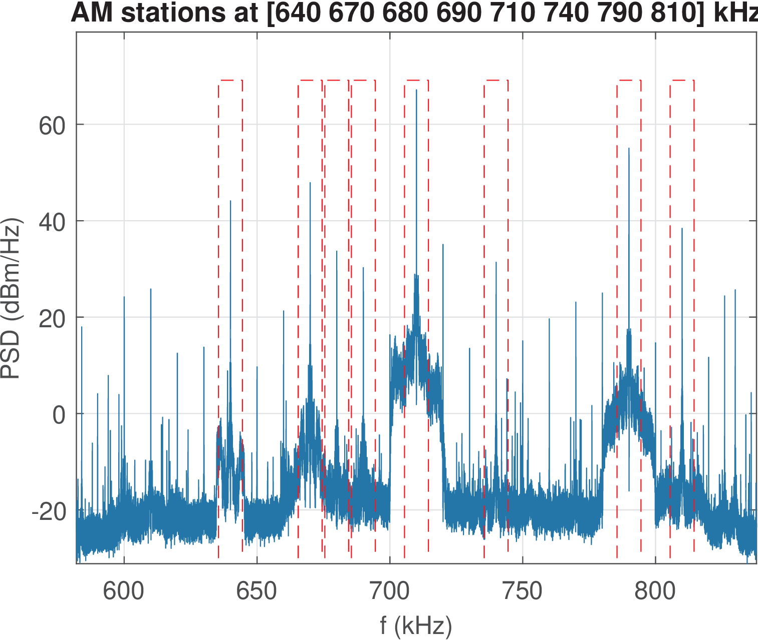
Figure 1.7: PSD of signal with frequency band from 582 to 838 kHz. Eight AM stations recorded in USA are identified.

The signal used to generate Figure 1.7 is described in Application 1.2. It has $BW = 256$ kHz and could potentially accommodate 25 AM radio stations spaced by 10 kHz. The eight stations with relatively clear (strong enough) signals are identified in Figure 1.7, with the strongest one being at the center frequency 710 kHz.⁵

1.4.1 Amplifiers

As suggested by Figure 1.7, a radio receiver has to use good filters in order to isolate the signal of interest from interferers and noise. Besides, the received signal often requires amplification.

Taking Figure 1.3 as reference, Figure 1.8 adds an amplifier just after the antenna. The AM signal of interest is assumed to be always centered at a radio frequency $f_{RF}$ and the local oscillator (LO) generates a frequency $f_{LO}$ that is ideally $f_{LO} = f_{RF}$ .

Figure 1.8: Simple radio architecture with a local oscillator (LO) generating a sinusoid with a fixed frequency for AM reception.

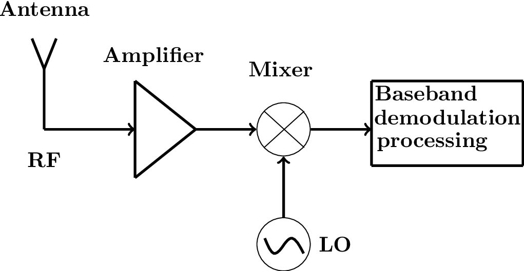
In Figure 1.8, the signal captured by the antenna, with a large bandwidth, would be entering the amplifier. This would increase the impact of the amplifier nonlinearities, such as intermodulation products, for example. Therefore, is it advisable to place a filter just after the antenna, which is called RF filter.

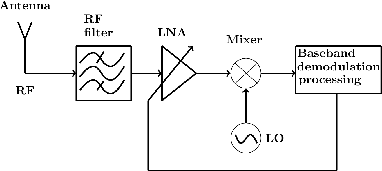
Another aspect that complicates the receiver design is that the receive signal power varies, and the amplifiers must have their gains adjusted accordingly. Hence, automatic gain control (AGC) blocks are commonly implemented based on a variable gain amplifier⁶ (VGA) and an arrow crossing the amplifier icon indicates its gain can be modified. As will be discussed in Section 1.7.6, instead of VGA, the amplifier in Figure 1.8 is called low-noise amplifier (LNA). The architecture with the RF filter and variable gain LNA is depicted in Figure 1.9, which indicates that the gain is controlled by the baseband demodulator.

Figure 1.9: Evolution of Figure 1.8, with RF filter and variable gain amplifier.

1.4.2 Advanced: Filtering issues

Most radio receivers use several filtering stages and shift the signal of interest to intermediate frequencies via mixers. This filtering process may include filters with high and low Q-factors (see Sections E.7.2.0 and E.9).

Filters with high Q-factor often have a fixed center frequency $f_{c}$ while filters with tunable $f_{c}$ have a more relaxed specification and lower Q. Components such as variable capacitors, tuning diodes, variable inductors, etc. can be used to tune $f_{c}$ of analog filters but there is a caveat if the filter has an approximately constant Q: its bandwidth will vary with $f_{c}$ . For example, when considering the commercial AM band as being fom 535 kHz to 1605 kHz, as in many countries, and a filter with $Q = 50$ , the bandwidth would vary from 10.7 kHz to 32.1 kHz, when varying $f_{c}$ from 535 kHz to 1605 kHz. In this case, $Q = 50$ is a good choice for AM stations with $BW = 10$ kHz in the vicinities of 535 kHz, but would lead to an excessively wide band for the upper frequencies.

1.4.3 Homodyne (direct conversion) receivers

Another issue to be addressed by the radio receiver is tuning to the desired center frequency $f_{c}$ . A conceptually simple strategy to have a tunable receiver is illustrated in Figure 1.10, where $f_{c}$ can be varied to select the desired RF band.

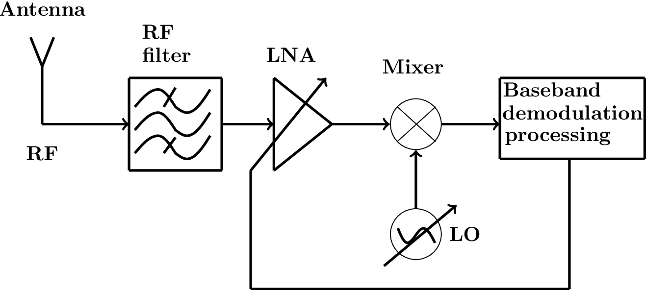
Figure 1.10: Homodyne receiver, which can be seen as a tunable version of Figure 1.9.

The architecture described in Figure 1.10 is called homodyne, direct-conversion receiver or zero-IF, because it does not use an intermediate frequency. However, the practical implementation of the homodyne receiver using analog processing has disadvantages when compared to the superheterodyne architecture, to be discussed in the sequel. But it should be noted that with the advent of fast ADC converters, which can digitize signals at the IF frequency, the homodyne architecture has been used in some software radio applications.

1.4.4 Homodyne, heterodyne and superheterodyne radio receivers

It should be noted that homodyne receivers “use” frequency heterodyning (mixing), and the jargon may sound confusing. It helps to understand the name “homodyne” receiver by contrasting it with the superheterodyne architecture.

A superheterodyne receiver uses an intermediate frequency (IF) such that the LO frequency is different from the RF frequency the radio should tune at. In retrospect, homodyne receivers still use heterodyning (mixing), but with a LO at the same frequency as the incoming signal. The name homodyne highlights that the LO and RF are the same frequency, which is also called “zero-IF conversion”. The name “heterodyne receiver” usually means a superheterodyne architecture where the LO is deliberately offset from RF, producing a nonzero IF. This is summarized in Table 1.1.

Table 1.1: Comparison between Homodyne and Heterodyne (Superheterodyne) Receivers.


Aspect	Homodyne (Direct Conversion)	Heterodyne (Superheterodyne)

Local oscillator (LO) frequency	Equal to the RF signal frequency (homo = same)	Different from the RF frequency (hetero = different)

Intermediate frequency (IF)	Zero (baseband, also called “zero-IF”)	Fixed, nonzero IF (e.g., 10.7 MHz in FM broadcast receivers)

Mixing operation	Still uses heterodyning (multiplication by LO), but shifts directly to baseband	Uses heterodyning to shift to a nonzero IF before further processing

Advantages	Simpler architecture, no IF filter needed	Excellent selectivity and image rejection with narrowband IF filtering

Challenges	DC offsets, LO leakage, I/Q imbalance	Requires additional IF filters, image-reject filter, more complex hardware

1.4.5 Advanced: Practical superheterodyne receiver

The goal here is to discuss the superheterodyne architecture, which is used in most AM receivers and in many other radio systems. Most of these systems support tuning to a desired RF frequency. But, for simplicity and sake of example, it is first assumed the system depicted in Figure 1.11.

Figure 1.11: Superheterodyne AM receiver without tuning capability.

The signal $m (t)$ to be demodulated in Figure 1.11 is centered at $f_{RF} = 1.4$ MHz and has ${BW}_{m} = 10$ kHz (not shown in the picture). By design, the IF frequency is 455 kHz, which is the most commonly used for AM broadcast receivers. Note that both RF and IF bandpass filters should have bandwidths not smaller than the ${BW}_{m}$ of the signal $m (t)$ , and in this specific case: ${BW}_{rf} = {BW}_{if} = {BW}_{m}$ .

As a complement to Figure 1.8, Figure 1.11 indicates that a possible baseband processing consists of an AM detector, which can be as simple as the circuit with a diode and first-order filter in Figure 1.6, and one or more audio amplifiers. Note that in this scheme, the AM detector incorporates the lowpass filter that is used in synchronous AM demodulation (Figure 1.3).

Two values of LO frequency $f_{LO}$ would center a replica of the PSD $S_{m} (f)$ of $m (t)$ at $f_{IF} = 455$ kHz: 945 and 1855 kHz. In fact, regarding the choice of $f_{LO}$ , the options $f_{LO} = f_{RF} + f_{IF}$ or $f_{LO} = f_{RF} - f_{IF}$ are called in the literature “high-side” and “low-side” injection, respectively. Due to practical aspects of analog circuits, the broadcast AM receivers use high-side injection. This is also the choice adopted in Figure 1.11. Note that in this case, the IF filter must attenuate (ideally eliminate) the replica of $S_{m} (f)$ located at 3,255 kHz.

The RF filter is the initial step for constraining the overall receiver BW to the minimum required. Assuming the background noise has white PSD, the smaller ${BW}_{RF}$ , the smaller the power of the noise entering the receiver. Using ${BW}_{RF} = {BW}_{m}$ is therefore pedagogical, but would require a filter with a relatively high Q-factor. As mentioned, high Q filters are more complex especially when the filter center frequency is tunable.

Considering now that tuning is a required feature, one could think of using a simple RF filter, with a bandwidth covering all frequencies of interest. For example, the non-tunable RF filter could have a passband from 535 kHz to 1605 kHz, to cover AM broadcast stations. The tuning could be done by varying $f_{LO}$ and using the IF filter to attenuate undesirable replicas. However, a mixer (as its names indicates) is susceptible to mix desired frequencies with their image frequencies.

An image frequency is any frequency other than the desired $f_{RF}$ that, if allowed to enter the mixer, will produce a cross-product frequency that is equal to $f_{IF}$ . For example, the RF filter in Figure 1.11 must attenuate the signal components in the vicinity of the image frequency 2310 kHz. The reason is that the mixer (with $f_{LO} = 1855$ ) will center a replica of these components at $2310 - 1855 = 455$ kHz. In other words, the frequency components at both $f_{RF} = 1400$ kHz and its image $f_{IM} = 2310$ kHz will be centered at $f_{IF} = 455$ kHz. Similar to aliasing in sampling, once an image frequency has been mixed into the output signal, it cannot be filtered or attenuated.

Example 1.6. Example of image frequencies in superheterodyning. In general, with high-side injection:

f_{IM} = f_{LO} + f_{IF} = f_{RF} + 2 f_{IF} .

(1.7)

Listing 1.2 illustrates how to obtain frequencies of interest associated to a mixer. In this case, LOh=1855,LOl=945,IMh=2310,IMl=490.

Listing 1.2: MatlabOctaveCodeSnippets/snip_digi_comm_mixerFrequencies.m

1RFfreq=1400; %RF frequency of interest (carrier) 
2IFfreq=455; %intermediate frequency, assumed: IFfreq < RFfreq 
3LOh=RFfreq+IFfreq %high-side injection LO frequency 
4LOl=RFfreq-IFfreq  %low-side injection LO frequency 
5IMh=RFfreq+2*IFfreq %image freq. for high-side (or, IMh=LOh+IFfreq) 
6IMl=RFfreq-2*IFfreq %image for low (or, alternatively,IMl=LOl-IFfreq)

From Listing 1.2, it can be seen that choosing a high value for $f_{IF}$ is beneficial for alleviating the requirements on the image rejection filter. However, the higher $f_{IF}$ , the more difficult it is to have analog amplifiers with high gain. Therefore, before a mixer, an image rejection filter should be positioned. $□$

Figure 1.12 illustrates a superheterodyne receiver architecture that supports tuning. In this case, the RF filter is called preselector because it is tunable and responsible for image rejection.

Figure 1.12: Superheterodyne AM receiver with the preselector filter responsible for image rejection.

Figure 1.12 illustrates the adoption of gang tuning, which means that adjustments of the center frequency of the preselector and the LO frequency are tied together (often mechanically, via the same tuning knob). As indicated by the relations in Listing 1.2, when the user tunes the radio, the frequencies $f_{RF}$ and $f_{LO}$ are simultaneously varied, always keeping a difference of $f_{IF}$ between them.

The literature in radio receivers is vast and there are several alternatives to the architectures discussed here. For example, a carrier synchronization scheme could be added to the architecture of Figure 1.12 to support synchronous demodulation. As another example, Figure 1.13 illustrates a superheterodyne architecture where the image rejection task is split between two filters and a second oscillator is used.

Figure 1.13: Alternative architecture to Figure 1.12 with an extra filter to perform image rejection and a second LO for converting from IF to baseband.

In the case of Figure 1.13, the first LO is responsible for bringing the desired signal spectrum to $f_{IF}$ and the second LO converts from $f_{IF}$ to zero.

⁵ The PSD in Figure 1.7 is specified in dBm/Hz, assuming that the signal samples are in volts. A calibration procedure of the measurement equipment is often necessary to actually obtain the amplitude in volts or other unit. Hence, it is very common to specify PSDs in dB/Hz given that the correct absolute power is unknown.

⁶ When the VGA gain can be controlled by e. g. a microcontroller, the VGA is called programmable-gain amplifier (PGA).