Examples of Analog Amplitude Modulation

1.3 Examples of Analog Amplitude Modulation

1.3.1 DSB-SC

Amplitude modulation can be performed by multiplying, via a mixer, the information signal $m (t)$ (corresponding to $x (t)$ in Figure 1.2) and a carrier $c (t) = cos (2 π f_{c} t + ϕ)$ to obtain the transmit signal

s (t) = m (t) cos (2 π f_{c} t + ϕ) .

(1.1)

The modulating signal $m (t)$ effectively changes the carrier amplitude over time. Consequently, the information of interest is “encoded” on the amplitude of $s (t)$ .

Coherent or synchronous demodulation allows to recover $m (t)$ from $s (t)$ in Eq. (1.1). The term “coherent” is used because this demodulation scheme requires generating the carrier $c (t)$ at the receiver by recovering both its frequency $f_{c}$ and phase $ϕ$ . In practice, the receiver uses estimates ${\hat{f}}_{c}$ and $\hat{ϕ}$ of the correct values $f_{c}$ and $ϕ$ .

To simplify the discussion, assume the ideal case of having ${\hat{f}}_{c} = f_{c}$ and $\hat{ϕ} = ϕ$ , with $c (t)$ perfectly regenerated at the receiver. In this case, $m (t)$ can be recovered by lowpass filtering the product $s (t) c (t)$ as follows:

m (t) = lowpass {s (t) cos (2 π f_{c} t + ϕ)},

which is illustrated in Figure 1.3.

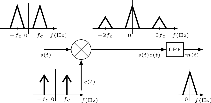
Figure 1.3: PSDs (bilateral) in coherent demodulation of a DSB-SC signal. An (ideal) lowpass filter can eliminate the replicas at $f = \pm 2 f_{c}$ .

This amplitude modulation scheme is called DSB-SC (double-sideband suppressed carrier) because the carrier “is not transmitted” and the bandwidth ${BW}_{rf}$ of $s (t)$ is twice the bandwidth ${BW}_{i}$ of the information signal.

In practice, several non-ideal circuits and algorithms impact the process suggested by Figure 1.3:

The receiver may estimate the correct frequency $f_{c}$ as $\hat{f_{c}} = f_{c} + Δ f$ instead, with the estimate error $Δ f$ being called frequency offset;
Similarly, the phase estimate $\hat{ϕ} = ϕ + Δ ϕ$ may incorporate a phase offset $Δ ϕ$ ;
A nonideal lowpass filter will attenuate the replicas at $f = \pm 2 f_{c}$ but not completely eliminate them. Besides, the nonideal filter will eventually distort the amplitude and phase of its input signal.

The reader is invited to explore the individual effects of each impairment using simulations.

1.3.2 SSB and VSB

Besides DSB-SC, there are several amplitude modulation schemes for analog signals, such as SSB, VSB and AM, for example. The SSB (single-sideband) and VSB (vestigial-sideband) are amplitude modulation schemes that, when compared to DSB schemes, reduce the required bandwidth to a value ${BW}_{rf} < 2 {BW}_{i}$ . The main interest here is in AM, which is a DSB scheme ( ${BW}_{rf} = 2 {BW}_{i}$ ) but, in contrast to DSB-SC, does not suppress the carrier. It is adopted by commercial broadcast stations and due to its popularity is simply called AM here.

1.3.3 AM

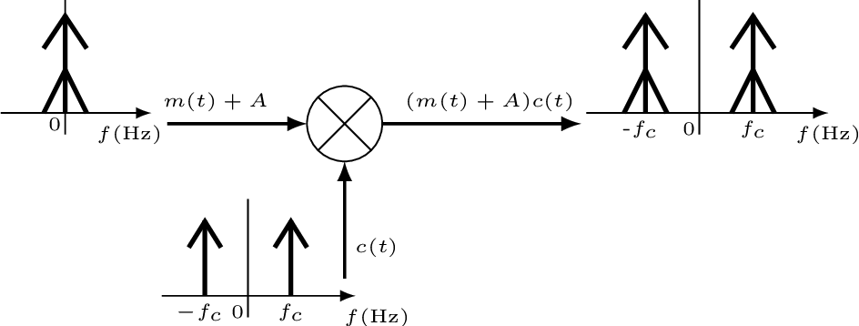
To enable envelope detection and, consequently, avoid coherent demodulation, AM is a modulation scheme in which a DC level $A$ is added to the information signal $m (t)$ before multiplication by the sinusoid carrier $c (t)$ . Different than the DSB-SC of Eq. (1.1), the AM transmit signal is

s (t) = (m (t) + A) cos (2 π f_{c} t + ϕ) .

(1.2)

The amplitude $A \geq - min {m (t)}$ is chosen to be not smaller than the magnitude of the negative peak of $m (t)$ , with $m (t)$ assumed to have mean $𝔼 [m (t)] = 0$ such that $min {m (t)}$ is indeed negative. This way the transmitter guarantees that $m (t) + A \geq 0$ , which allows $m (t)$ to be recovered by a relatively cheap envelope detection of the received version of $s (t)$ . An AM receiver signal can recover $m (t)$ in Eq. (1.2) using coherent demodulation, but the envelope detection scheme is simpler and cheaper to implement.

In designing an analog amplitude-modulation system, one must choose between a more energy-efficient DSB-SC scheme and a simpler AM scheme that allows envelope detection at the receiver but requires the transmitter to spend additional power transmitting the carrier.

Advanced: PSD of AM signals

Assuming $m (t)$ is zero-mean and following the reasoning discussed in Section F.5.5, the AM signal of Eq. (1.2) has PSD given by

S_{AM} (f) = \frac{1}{4} [S_{m} (f + f_{c}) + S_{m} (f - f_{c})] + \frac{A^{2}}{4} [δ (f - f_{c}) + δ (f + f_{c})],

(1.3)

where $S_{m} (f)$ is the PSD of $m (t)$ .

Using Eq. (F.20) to integrate Eq. (1.3) over frequency shows that the parcel $\frac{A^{2}}{4} [δ (f - f_{c}) + δ (f + f_{c})]$ that “transmits the carrier” corresponds to an overhead that consumes power $P_{c} = A^{2} ∕ 2$ . This is consistent with the fact that this parcel in time-domain is $A cos (ω_{c} t + ϕ)$ and $A^{2} ∕ 2$ is the power of a cosine.

Figure 1.4 illustrates that the added DC level appears as an impulse $A^{2} δ (f)$ in the PSD of $(m (t) + A)$ , which is shifted to the frequencies $\pm f_{c}$ by the mixer. It should be contrasted with the DSB-SC PSD at the right of Figure 1.2, which does not have the impulses corresponding to the DC level.

Figure 1.4: Bilateral PSDs of AM signal and mixer inputs. The level $A$ appears originally as an impulse at the DC of the baseband signal and is shifted by the mixer to frequencies $\pm f_{c}$ .

Example 1.2. Example of PSD mask for AM transmission. Figure 1.5 gives an example of a possible RF PSD mask for AM transmission² with PSD values given in dBc, i. e., with respect to the carrier power. The mask in this example indicates that within 10.2 kHz from the channel frequency, the PSD cannot exceed $- 25$ dBc.

Figure 1.5: Example of RF mask adopted for regulating AM transmission.

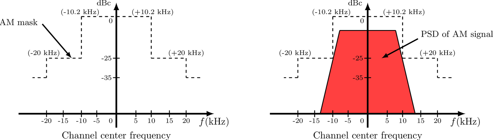
PSD masks are imposed by regulatory agencies and indicate the limits but, for example, many AM broadcasters use BW smaller than 10 kHz such as 5 kHz. $□$

Conceptually, the AM signal can be demodulated with the schemes depicted in Figure 1.6 using either digital or analog signal processing.³ In practice, several extra processing stages must be added, as will be discussed in Section 1.4.

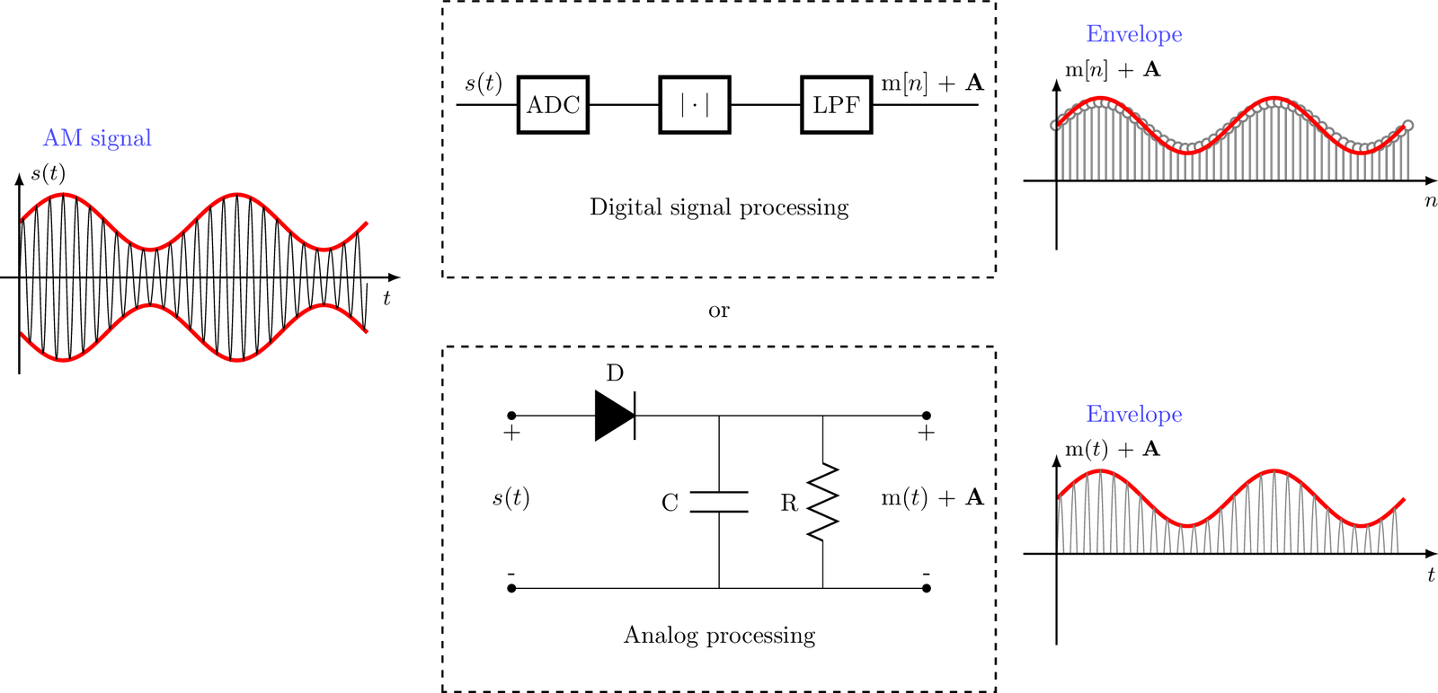
Figure 1.6: High-level description of possible schemes for AM demodulation.

Example 1.3. The carrier frequency must be high enough. The signals in Figure 1.6 can be generated with Listing 1.1 (only the first lines are shown here).

Listing 1.1: MatlabOctaveCodeSnippets/snip_digi_comm_amSignals.m

1N=80; %total number of samples used in the simulation 
2Np=8, Ns=50; %period of carrier and information signal, respectively 
3Ts=0.25; %sampling period in seconds 
4n=0:N-1; t=n*Ts; %abscissas in n and t, respectively 
5m=sin(2*pi/Ns*n); %information signal 
6A=1.8; %DC level 
7x=(m+A).*cos(2*pi/Np*n); %AM signal

One should observe that the carrier frequency must be high enough to have the AM demodulation working properly. The reader is invited to change the period of the carrier frequency in Listing 1.1 from 2 to 16 samples, and observe the results. $□$

Applications 1.1 and 1.2 further discuss AM.

Advanced: AM modulation index and power overhead

How large is the AM power overhead is controlled by the modulation index $h$ , which is a measure of how much the peak amplitude of $s (t)$ in Eq. (1.2) varies with respect to the unmodulated amplitude $A$ (i. e., $m (t) = 0$ in Eq. (1.2)). With $m (t)$ being zero-mean and having the same amplitude values for the positive and negative peaks (i. e., $max {m (t)} = - min {m (t)}$ ), $h$ is given by

h = \frac{max {m (t)}}{A},

(1.4)

and often expressed as a percentage. To allow envelope detection, a modulation index not larger than 100% is required.⁴ The impact of $h$ in the AM power overhead is discussed in the sequel.

Example 1.4. AM power overhead when the information signal is a sinusoid. To simplify the analysis, assume that $m (t) = A_{m} cos (2 π f_{m} t)$ is a pure sinusoid with peak value $A_{m} = hA$ and frequency $f_{m} < f_{c}$ . In this case, using Eq. (A.10), one can calculate that the parcel $m (t) cos (ω_{c} t + ϕ)$ of Eq. (1.2) has power $P_{m} = A_{m}^{2} ∕ 4 = A^{2} h^{2} ∕ 4$ . Hence, the total power $P_{AM} = P_{m} + P_{c}$ of the AM signal, in the case of $m (t)$ being a sinusoid, is:

P_{AM} = P_{m} + P_{c} = \frac{A^{2} h^{2}}{4} + \frac{A^{2}}{2} = \frac{A^{2}}{2} (1 + \frac{h^{2}}{2}) = P_{c} (1 + \frac{h^{2}}{2}) .

(1.5)

As mentioned, the maximum $h$ for envelope detection is 100% and, in this case, the AM power overhead $P_{c} ∕ P_{AM}$ is $2 ∕ 3$ such that the signal parcel that carries information corresponds to only 33.3% of the transmit power. In practice, $h < 1$ and the AM power overhead would be larger than $2 ∕ 3$ for a sinusoidal $m (t)$ . $□$

Example 1.5. AM power overhead when the information signal has amplitude normally distributed. As another example, consider when the amplitude of $m (t)$ is distributed according to a Gaussian $N (μ, σ^{2})$ with $μ = 0$ and variance (power) $σ^{2}$ . After multiplication by the carrier cosine, $P_{m} = σ^{2} ∕ 2$ , as discussed in Section F.5.5. To relate $P_{m}$ and $P_{c}$ , assume that the peak value of $m (t)$ is $3 σ$ , such that from Eq. (1.4), $σ = hA ∕ 3$ .

P_{AM} = P_{m} + P_{c} = \frac{σ^{2}}{2} + \frac{A^{2}}{2} = \frac{h^{2} A^{2}}{18} + \frac{A^{2}}{2} = \frac{A^{2}}{2} (1 + \frac{h^{2}}{9}) = P_{c} (1 + \frac{h^{2}}{9}) .

(1.6)

In this case, even $h = 1$ would lead to $P_{m} = 0.1 P_{AM}$ and a 90% power overhead. $□$

Many methods have been investigated to decrease the AM power overhead such as “companding”, which is similar to the strategy used in PCM with $μ$ or A-law to compress (at Tx) and expand (at Rx) the amplitude of $m (t)$ .

² Adapted from the document NRSC-2-B made available by the National Radio Systems Committe (NRSC), USA, at [ url5nrs]. Check also the document NRSC-G100-A.

³ In the examples of Figure 1.6, the diode-based half-wave rectification in the analog version differs from the digital counterpart in the sense that the latter implements a full-wave rectification via the $|⋅|$ function. A command such as s(s<0)=0 would simulate a half-wave rectifier in Matlab/Octave. With proper filtering, both rectifications can recover the signal envelope.

⁴ The script MatlabOctaveCodeSnippets/snip_digi_comm_amIndexModulation.m provides an example for which Eq. (1.4) is not valid.