1.8  Applications

Application 1.1. Creation and demodulation of AM signals. The goal here is to create a multiplex signal with $N$ ($N=4$ is assumed) AM signals and demodulate it. The code can be found at folder Applications/AMDemodulation of the companion software.

The signal that goes in each AM channel can be generated by the user in two steps: 1) First the user records $N$ wav files using $F_s=44100$ Hz, name them as explained in file ak_resampleFiles.m, and runs this script, which converts the files to $F_s=8$ kHz. 2) The script ak_amCreateMultiplexedSignals.m shifts the $N$ signals in frequency, sums them to create the multiplexed signal and stores this signal at file amMultiplexedSignals.wav. This script requires information about the IF frequency (Fc_if variable) and the RF frequency of each AM signal.

Then, the script ak_amDemodulation.m implements the demodulation process for the $N=4$ signals multiplexed in amMultiplexedSignals.wav.

The scripts can be modified to use other frequencies, bandwidths, etc. Two tasks are suggested in the sequel.

The first task is to implement code to estimate the SNR between the original and demodulated signals. This will require aligning the signals, as illustrated in Listing C.35, discussed in Section C.13. The reader may also look at Application E.10. More specifically, two baseband signals $x_1[n]$ and $x_2[n]$ should be recorded. These signals should be modulated and multiplexed to compose a single signal $s[n]$ with sampling frequency $F_s=44.1$ kHz. The two AM signals should comply with the PSD mask described in Figure 1.5. Generate a figure showing the PSD with superimposed masks at the carrier frequencies.

The demodulation of $s[n]$ should recover the respective estimates ${\widehat{x}}_1[n]$ and ${\widehat{x}}_2[n]$. A perfect gain scaling can be assumed, in which the receiver knows the power of $x_1[n]$ and $x_2[n]$ . With this information, the amplitudes of ${\widehat{x}}_1[n]$ and ${\widehat{x}}_2[n]$ can be scaled to force the resulting signals to have the same power as their original versions.

The function filtfilt.m cannot be used (use filter.m instead) because we want to rely only on causal systems. After time-alignment, the two SNR values, between the original $x_i[n]$ and its estimate ${\widehat{x}}_i[n]$, $i=1,2$, should be calculated. The system must be designed such that the SNR is larger than 20 dB. Estimate the computational cost as the number $N_{}$

ma$ofmultiplicationsplusadditionsofthefilteringoperationsinthedemodulator(donottakeinaccountthealignmentprocedure,forexample).Minimize$N_ma$whileachieving$SNR$\ge 20$ dB. Inform the delay of the overall system (modulator and demodulator) in seconds.    $\square$

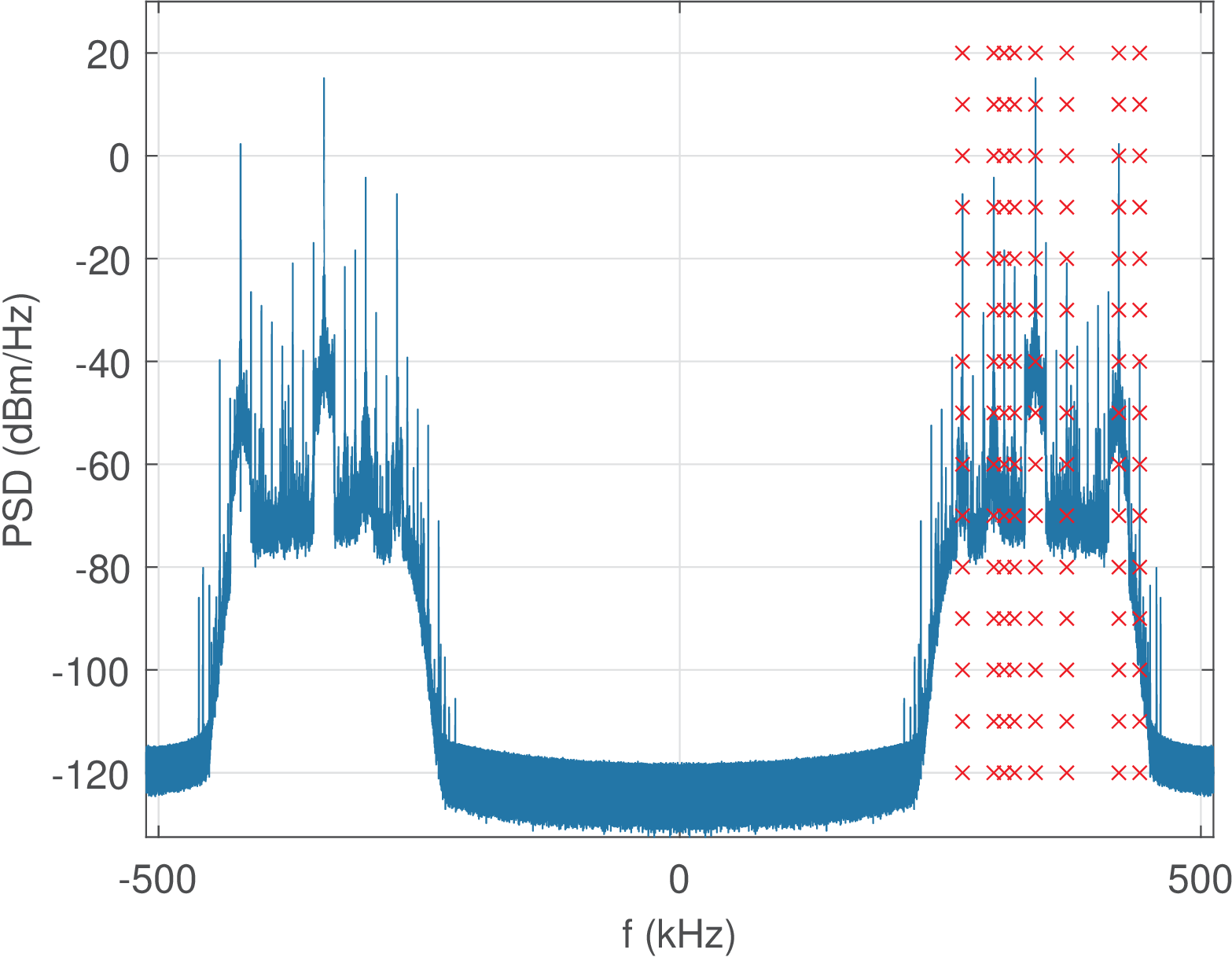
Application 1.2. Demodulation of the digitized signal corresponding to multiplexed real-life AM stations. The experiment suggested here uses the companion file am_real.wav (around 20 MB).¹⁷ In summary, a software radio platform was tuned to capture a radio frequency (RF) band centered at $f_c$ with bandwidth BW. This digitized signal was used to generate the signal $x[n]$ stored in am_real.wav, as described in Application 3.2.

The real-valued signal $x[n]$ corresponds to approximately 11 seconds sampled at $F_s=1,024$ kHz. It has ${\mathrm{\text{BW}}}_{\mathrm{\Omega }}=1.57$ rad and is centered at ${\mathrm{\Omega }}_c=2\pi ∕3$ rad. Using Eq. (C.36), these frequencies correspond to $\mathrm{\text{BW}}=256$ kHz and $f_c=341.33$ kHz, respectively. Figure 1.18 shows the PSD of $x[n]$. The 8 AM stations are located at approximately $[271,301,311,321,341,371,421,441]$ kHz (to be more accurate, add $1∕3$ kHz to these frequencies). The second and third stations are only 10 kHz apart, as well as the third and fourth.

The script ak_amDemodulateDigitizedAMSignal.m can be used to demodulate the AM stations represented in signal $x[n]$ of the companion file am_real.wav. Some lines of this code, corresponding to seven processing steps, are shown in Listing 1.12, where rx is the original signal read from am_real.wav.

35    r = rx.*carrier(:); %1) frequency downconversion 
36    r = filtfilt(B1,A1,r); %2) filter to eliminate image 
37    [r,h4]=resample(r,1,2,10); %3) to Fs/2, filter order=40 
38    r = filtfilt(B2,A2,r); %4) filter again for improved performance 
39    [r,h5]=resample(r,Fsfinal,Fs/2,20); %5) to Fsfinal, order=2560 
40    m=abs(r); m=m-mean(m); %6) get magnitude (envelope), subtract DC 
41    m=filtfilt(B3,A3,m); %7) better filter envelope at Fsfinal
  

The demodulation uses two resampling steps to decrease the original $F_s=1,024$ kHz to 8 kHz. The motivation is to decrease the computational cost and facilitate the filtering operations. The first resampling corresponds to step 3 in Listing 1.12 and decreases $F_s$ by a factor of two. The second resampling happens in step 5 and changes the sampling frequency from 512 kHz to 8 kHz. The function resample.m automatically designs a lowpass filter to avoid aliasing. In the first resampling, the FIR filter h4 has order 40, while the second resampling used a filter (h5) of order $2,560$.

Besides the filtering executed by resample.m, three additional filtering operations were performed using IIR filters in steps 2, 4 and 7. To obtain zero phase, the noncausal filtfilt.m operation was adopted. The whole procedure is just an example and other filters and functions could be used. In the sequel, the PSD after each step of demodulating the AM station centered at $341.33$ kHz is shown and discussed. This is the fifth station in Figure 1.18 and it is in the center of the band of 256 kHz.

Figure 1.19 shows the PSDs after steps 1 and 2. The carrier used for frequency downconversion was $e^{-j(2\pi ∕3)n}$ rad. One thing to note is that the spectrum replica at positive frequencies in Figure 1.18 is moved to DC while a replica originally at negative frequencies shows up at its right. This is due to the periodicity of the spectrum of $x[n]$.

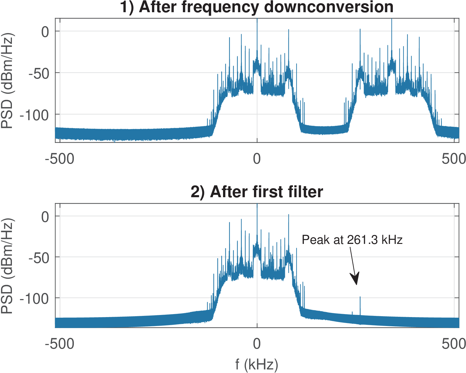
Figure 1.18 shows replicas that are centered in ${\mathrm{\Omega }}_{-1}=-2\pi ∕3$ and ${\mathrm{\Omega }}_1=-2\pi ∕3$ rad. The frequency shift by $2\pi ∕3$ moves them to ${\mathrm{\Omega }}_{-1}-2\pi ∕3=-4\pi ∕3$ and ${\mathrm{\Omega }}_1-2\pi ∕3=0$. While the latter is centered at DC, the replica originally ${\mathrm{\Omega }}_{-1}$ “disappears” from the chosen visualization range of $[-\pi ,\pi [$ because its highest frequency is $-4\pi ∕3+{\mathrm{\text{BW}}}_{\mathrm{\Omega }}∕2=-3.4$ rad. However, the replica located at ${\mathrm{\Omega }}_{-2}=-2\pi ∕3+2\pi$, which was not shown in Figure 1.18, appears at ${\mathrm{\Omega }}_{-2}-2\pi ∕3=2.09$ rad in Figure 1.19. All this reasoning can be done in Hertz instead of radians. On purpose, both Hz and rad are used here to familiarize the reader with their connection via Eq. (C.36).

The filtering in step 2 aims at eliminating the replica at $2.09$ rad. Note that the result still shows a peak at 261.3 kHz, as indicated in Figure 1.19. It corresponds to the second strongest peak when considering the whole bandwidth of the AM stations but becomes prominent because it is closer to the filter cutoff frequency than the strongest peak and, therefore, less attenuated. This same peak shows up in Figure 1.20 at frequency $261.3-512=-250.7$ kHz as discussed in the sequel.

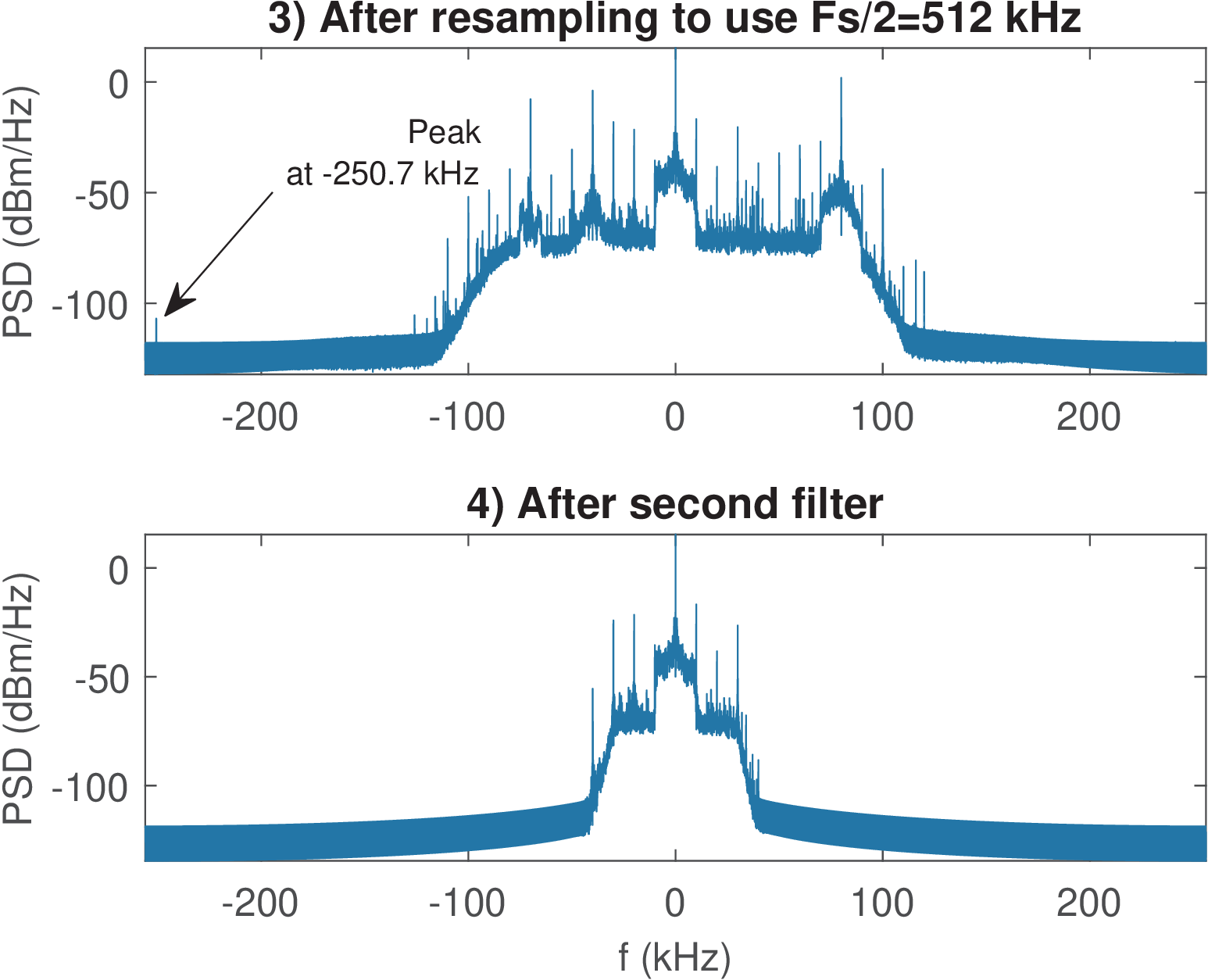
Figure 1.20 shows the PSD after steps 3 and 4: resampling to $F_s∕2=512$ kHz and additional filtering. The function resample.m in step 3 implements (using FIR h4) a lowpass filtering with cutoff frequency $\pi ∕2$ rad and then decimates by 2. The decimation stretches the frequency axis such that $[-\pi ,\pi ]$ corresponds now to $[-256,256[$ kHz and creates replicas that, in Hz, are located at multiples of 512 kHz. Hence, after getting attenuated by the filter h4, the peak at 261.3 kHz in Figure 1.19 shows up at $261.3-512=-250.7$ kHz in Figure 1.20. The $10^{\mathrm{\text{th}}}$ second filter has a cutoff frequency of 30 kHz and significantly attenuates the frequencies outside this range.

Figure 1.21 shows the PSDs after steps 5, 6 and 7. Step 5 converts the sampling frequency from 512 to 8 kHz, while 6 obtains the “envelope” m of the received signal r already filtered and centered at DC. The third filter has a cutoff frequency of only 1.5 kHz, as indicated by the dashed lines in Figure 1.21.

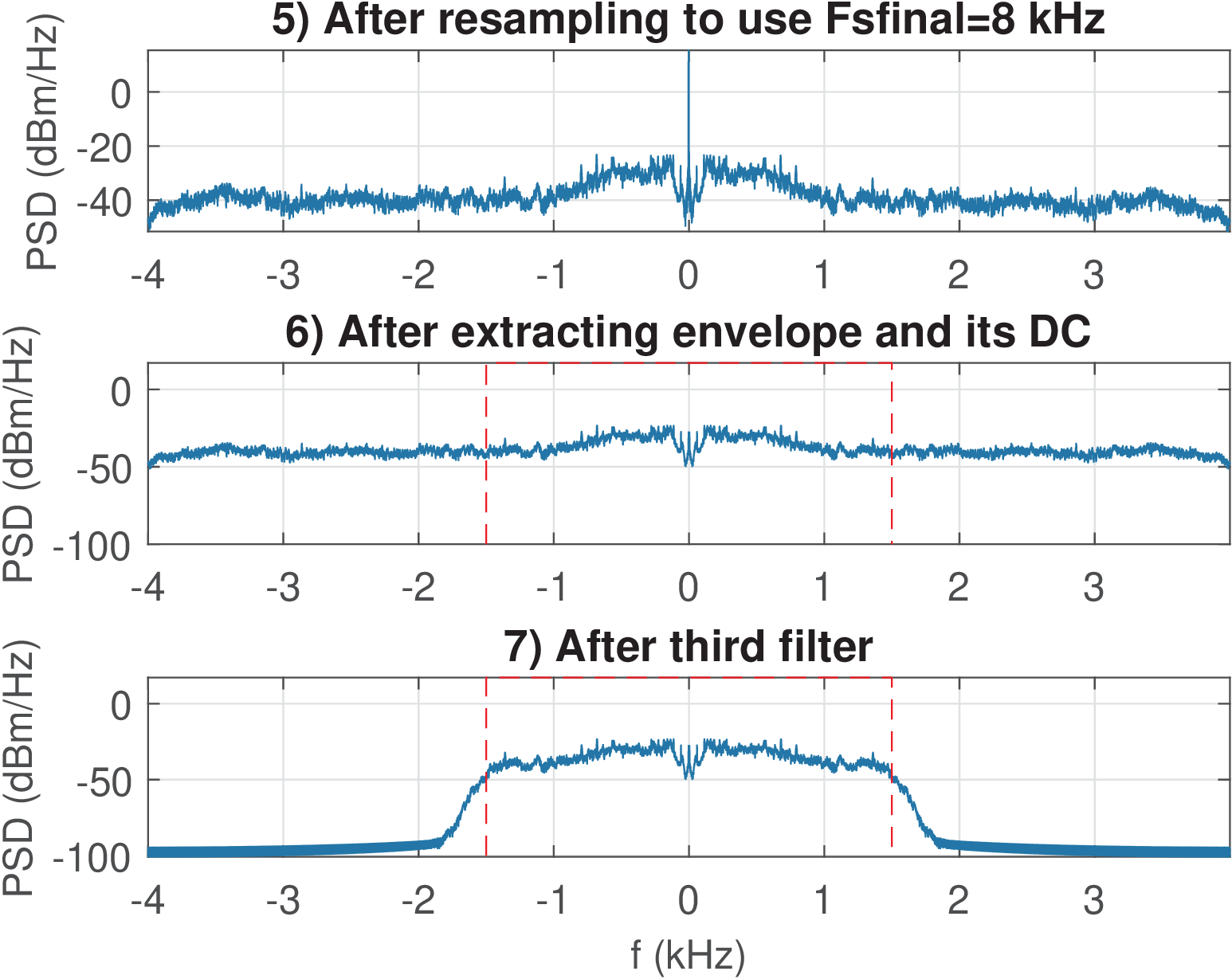
The final PSD (bottom plot of Figure 1.21) indicates that all the resampling and filtering steps led to strong attenuation of out-of-band frequencies. Simpler procedures could be adopted without noticeable distortion.

For completeness, note that $x[n]$ is centered at frequency $f_c=341.33$ kHz but before its A/D conversion, it was located at an RF frequency of 710 kHz. The acquisition hardware and further processing created a frequency difference of $368.67$ kHz between the RF and the “DSP” frequency $f_c$. Hence, the corresponding band at RF was $710\pm \mathrm{\text{BW}}∕2$, which corresponds to $[582,838]$ kHz. These RF frequencies were mapped to DSP frequencies in $x[n]$ corresponding to $[240.67,496.67]$ kHz. For example, the frequencies $341.33$ and 371.33 kHz of $x[n]$ correspond to RF frequencies of 700 and 740 kHz, respectively. This is further explained in Application 3.2.   $\square$

Application 1.3. Transmission of AM over simulated AWGN channel. Record your own AM signals $x_1[n]$ and $x_2[n]$, and multiplex them into a signal $x[n]$. Both $x_1[n]$ and $x_2[n]$ must have an initial sampling frequency of 8 kHz and $x[n]$ a sampling frequency of 44 kHz. The carrier frequencies adopted for $x_1[n]$ and $x_2[n]$ must be 7 and 16 kHz, respectively. All three signals $x_1[n]$, $x_2[n]$ and $x[n]$ must be saved in WAV files. The multiplex signal $x[n]$ must be transmitted through an AWGN channel that adds noise $\nu [n]$, generating a received signal $\widehat{x}[n]$. The noise power $P_{\nu }$ is chosen such that one can control the channel SNR, defined as ${\mathrm{\text{SNR}}}_c=P_x∕P_{\nu }$, where $P_x$ is the power of $x[n]$. Write the software to demodulate $\widehat{x}[n]$ and write ${\widehat{x}}_1[n]$ and ${\widehat{x}}_2[n]$ as WAV files. The goal is to obtain demodulated signals ${\widehat{x}}_1[n]$ and ${\widehat{x}}_2[n]$ with a good quality, but you cannot use non-causal processing (as done in filtfilt.m, for instance). The demodulation should be assessed subjectively by listening ${\widehat{x}}_1[n]$ and ${\widehat{x}}_2[n]$, and also via ${\mathrm{\text{SNR}}}_d=({\mathrm{\text{SNR}}}_1+{\mathrm{\text{SNR}}}_2)∕2$, where each ${\mathrm{\text{SNR}}}_i,i=1,2$, is given by ${\mathrm{\text{SNR}}}_i=𝔼[|x_i[n]{|}^2]∕𝔼[|x_i[n]-{\widehat{x}}_i[n]{|}^2]$. A plot should be generated, showing how ${\mathrm{\text{SNR}}}_d$ varies with ${\mathrm{\text{SNR}}}_c$, considering an abscissa ${\mathrm{\text{SNR}}}_c$ in the range $[-5,30]$ dB. Recall that after filtering, the signals may need to be synchronized (realigned in time).    $\square$

Application 1.4. Transmission of AM over the sound board. Transmit two AM signals $x_1(t)$ and $x_2(t)$, both with a bandwidth of 4 kHz, over an audio cable using PC sound systems working at $F_s=44.1$ kHz. The two signals must be multiplexed into a signal $x(t)$ at the “carrier” frequencies of 7 and 16 kHz, and transmitted simultaneously. The multiplex signal $x(t)$ should be pre-computed and saved as a WAV file. The transmitter should use the Audacity software to continuously transmit $x(t)$ on a loop. An audio cable is the channel between transmitter and receiver, which can be implemented using one or two PCs, depending on their sound board capabilities. The audio gains should be properly adjusted beforehand. The receiver should be implemented on Octave or Matlab. The receiver routine should acquire a pre-specified duration $T$ of the received signal $\widehat{x}(t)$ (e. g. 4 seconds), demodulate it and playback ${\widehat{x}}_1(t)$ and then ${\widehat{x}}_2(t)$ over the receiver sound system. These three steps should be repeated in a loop. The goal is to obtain demodulated signals ${\widehat{x}}_1(t)$ and ${\widehat{x}}_2(t)$ with a good quality. Advanced users can implement a time-alignment procedure based on cross-correlation and estimate the SNR between $x_i(t)$ and their respective demodulated versions ${\widehat{x}}_i(t),i=1,2$.   $\square$

Application 1.5. Synchronization of GSM handsets (adapted from [ url5gra]). The GSM base station must use¹⁸ a frequency source with absolute accuracy better than 0.05 ppm for both RF frequency generation and clocking the symbols $m_i$. Considering the 900 MHz GSM band, an error of 0.05 ppm is 900e6/1e6*0.05=45 Hz and, in the 1800 MHz band, it is 90 Hz. This high level of accuracy can be achieved by, e. g., temperature-compensated voltage-controlled crystal oscillators (TCVCXO) or oven-controlled crystal oscillators (OCXO), which typically cost more than a hundred American dollars. To lower the cost, a GSM handset may use a less accurate oscillator than the base station’s, with an accuracy of 20 ppm, for example (18000 and 36000 Hz for the 900 and 1800 MHz bands, respectively).

Therefore, the base station periodically sends a beacon signal for helping the handsets to synchronize their signals. When the handset is turned on, it searches for the beacon to adjust its internal signals for timing and carrier recovery. After the initial synchronization, keeping the signals locked still requires processing. For example, the Doppler shift from a vehicle moving at 150 km/h is approximately 0.15 ppm and demands phase-locked loops (PLL) or other processing for synchronization.

For the sake of comparison, the IEEE 802.15.4 standard allows $\pm 40$ ppm, which corresponds to approximately $\pm 100$ kHz for a carrier of 2.4835 GHz. Investigate the requirements for distinct communication standards and the price for the respective oscillators.    $\square$

Application 1.6. The use of heterodyning in spectrum analyzers. Spectrum analyzers are very important when evaluating RF circuits. Broadly, they can be categorized as analog or digital. But many modern equipment are hybrids, using concepts of both schemes.

The architecture of a digital analyzer is basically composed of a lowpass filter, ADC converter operating at $F_s$ and an FFT. In this case, the sampling frequency $F_s>2f_{\mathrm{\text{max}}}$ imposes the limit of the supported maximum input signal frequency $f_{\mathrm{\text{max}}}$. To expand the range of supported frequencies, spectrum analyzers use heterodyning.

A spectrum analyzer can use a mixer and a tunable bandpass filter, in a gang-tuning scheme, to sweep the input signal spectrum. But, as discussed in Section 1.4, filtering directly in RF would cause problems such as, given the filter’s Q-factor, having distinct bandwidths as the center frequency varies. Therefore, analog spectrum analyzers also use an intermediate frequency (IF) and, similar to Figure 1.12, the IF filter determines the so-called analyzer’s resolution BW (or RBW). A simplified block diagram is depicted in Figure 1.22. In this case, the video signal is the input to an analog output display.

Hybrid spectrum analyzers use fast ADCs that can convert signals directly at IF. For example, an ADC with $F_s=96$ MHz can be used to digitize a RF signal of bandwidth 20 MHz centered in 1.8 GHz. Due to heterodyning, the input frequency range is independent of the ADC rate.

The RBW of an FFT-based spectrum corresponds to the FFT resolution in Eq. (D.37) and Eq. (D.38). Hence, the RBW of an FFT-based spectrum is determined by the length of the digitized and stored (in RAM memory) signal. To complement the many good textbooks in spectrum analysis, the reader is invited to read the material made available by manufacturers.¹⁹   $\square$

Application 1.7. Digital down-converter (DDC) and up-converter (DUC) as used in software radios. A software-defined radio architecture may have the ADC close to the antenna, digitizing almost directly the RF signal. This way, the digitized RF signal itself would already be processed with DSP techniques. However, with current technology, it is more common to use a heterodyne module and digitize the signal at an IF or even apply direct conversion from RF to baseband and digitize the signal at baseband. When the (real) signal is digitized at an IF, a digital down-converter (DDC) is often used to create a baseband complex version centered at zero frequency. The DDC uses a numerically-controlled oscillator (NCO) and can also make a “fine tuning” of the signal center frequency in a stage where the signal is almost at baseband but there is an offset from zero.

The digital up-converter (DUC) performs frequency upconversion. Both DDC and DUC are used in the USRP software radio architecture [ url5usr].    $\square$