1.2  Heterodyning via mixers

Before discussing amplitude modulation, it is useful to understand heterodyning, the process of combining frequencies to create new ones. Heterodyning is also understood as synonymous of frequency conversion because it is widely used to shift a signal of interest to a new frequency range. In its simplest form, it consists in multiplying two input signals $x(t)$ and $c(t)$ as depicted in Figure 1.1. The multiplier is a linear but time-variant (LTV) device and is called mixer. Recall from Result E.1 that linear and time-invariant (LTI) systems cannot create new frequencies, but the mixer is not LTI.

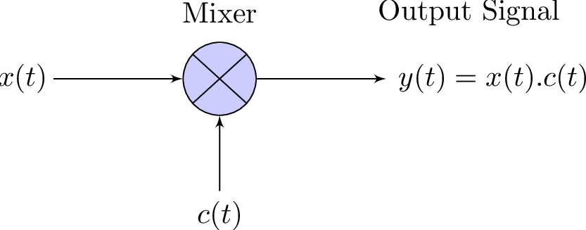
As indicated by Eq. (A.11), when $x(t)$ and $c(t)$ in Figure 1.1 are sinusoids with positive frequencies $f_x$ and $f_c$, the output $y(t)=x(t)c(t)$ of the mixer is a sum of two sinusoids with frequencies $f_x+f_c$ and $|f_x-f_c|$. In practice, mixers are not perfect multipliers and generate harmonics of the input frequencies and intermodulation distortion (IMD).

The carrier signal $c(t)$ of Figure 1.1 is often a sinusoid and $x(t)$, the signal of interest, can be modeled, for example, as a realization of a WSS random process $X(t)$ with PSD $S_x(f)$. In this case, the process at the mixer output has PSD given by e. g. Eq. (F.34). The mixer input can also be modeled as a deterministic signal. For instance, if $x(t)$ is non-random and periodic, $S_x(f)$ can be obtained with Eq. (F.29) and then Eq. (F.34) gives the output PSD.

Example 1.1. Example of unilateral PSDs at inputs and output of a mixer. Figure 1.2 illustrates the associated PSDs in two distinct cases.¹

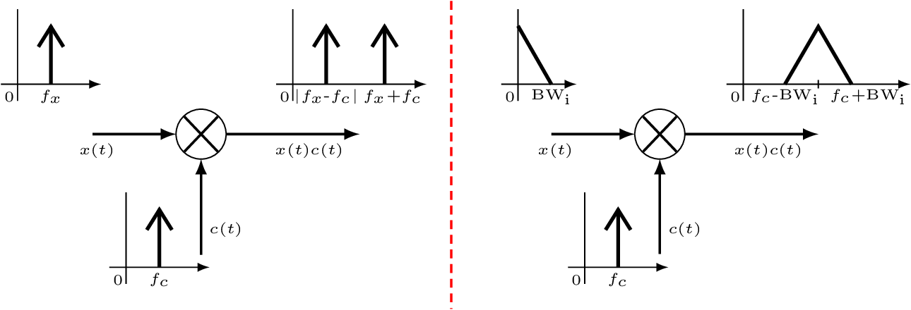
The left plot in Figure 1.2 corresponds to the case in which $x(t)$ is a sinusoid. Considering e. g. $f_x=10$ and $f_c=15$, the output is a sum of two sinusoids with frequencies 5 and 25. The signals are real-valued, therefore only the positive frequencies are shown (the unilateral PSD representation is adopted instead of the bilateral). But the negative frequencies must be take in account to properly interpret the results. Note also that, swapping the frequency values and assuming for instance: $f_x=15$ and $f_c=10$, also leads to the same result.

The right plot in Figure 1.2 corresponds to having the information signal $x(t)$ as the realization of a WSS process with a bandwidth ${\mathrm{\text{BW}}}_{\mathrm{\text{i}}}$. As will be discussed in the sequel, the output signal is called double-sideband because it has a bandwidth $2{\mathrm{\text{BW}}}_{\mathrm{\text{i}}}$, which is twice the bandwidth of $x(t)$.   $\text{□}$