Link Budget

1.7 Link Budget

The analysis of gains and losses along a transmission path is called link budget and allows to quantify the link performance. It is typically a high-level description of a communication system and takes in account the attenuation over the medium (path loss), the antenna gains (often specified in dBi, the gain with respect to the hypothetical isotropic antenna), amplifiers, attenuators, etc. For example, a link budget with powers in dBm can be expressed generically by

P_{Rx} (dBm) = P_{Tx} (dBm) + gains (dB) - losses (dB),

(1.16)

where $P_{Rx}$ and $P_{Tx}$ are receive and transmit powers, respectively, which can be specified in dBW or any other absolute power unit in dB scale.

There are many sophisticated models to be used in link budget calculations (e. g., for propagation over a given medium) and also simplified expressions such as the free-space path loss (used in the popular Friis transmission equation). These are briefly discussed in this section, but first the concepts of sensitivity and link margin are highlighted.

1.7.1 Sensitivity and link margin

The receiver sensitivity is the minimum detectable input power $P_{min}$ of the signal to produce an “acceptable” output. The notion of “acceptable” depends on many aspects, such as the modulation scheme and can be specified, for instance, by a minimum ${SNR}_{min} = P_{min} ∕ P_{n}$ , where $P_{n}$ is the total noise power at the receiver.

In digital communications, ${SNR}_{min}$ can be obtained from standards or, for example, link-level simulations that indicate the SNR value to restrict the bit error rate to the maximum allowed value.

The difference (in dB scale) between the receiver sensitivity and the actual received power is called the link margin.¹² For example, a reliable wireless link can eventually require a minimum margin of 10 dB.

A discussion about receiver sensitivity in the context of 3GPP mobile communications, can be found at [ url5sen]. This application note indicates reference sensitivity levels in the range of $- 100$ to $- 91$ dBm for LTE.

1.7.2 Free-space propagation

Assuming the transmitter antenna radiates isotropically,¹³ the power density on the surface of a sphere with radius $d$ is $P_{Tx} ∕ (4 π d^{2})$ , where $P_{Tx}$ is the transmit power expressed in watts (linear units, not in dB). Completing this simplified model with a receiver antenna with effective area $A_{Rx}$ , the received power is then

P_{Rx} = \frac{P_{Tx}}{4 π d^{2}} A_{Rx} .

(1.17)

Real antennas are not isotropic radiators, and the transmit gain $G_{Tx}$ must be taken into account to estimate the received power $P_{Rx} = (P_{Tx} G_{Tx} A_{Rx}) ∕ (4 π d^{2})$ , where $G_{Tx}$ is the transmit antenna gain (dimensionless, referenced to isotropic). The product $G_{Tx} P_{Tx}$ is called equivalent isotropically radiated power (EIRP). In some references, the EIRP includes cable losses between the transmitter and the antenna, but this convention is not used here. The EIRP in dB, is given by

EIRP (dB) = 10 {log}_{10} (G_{Tx}) + 10 {log}_{10} (P_{Tx}),

(1.18)

where $P_{Tx}$ is in watts and $G_{Tx})$ is dimensionless (linear gain).

Note that a passive circuit working as an antenna could not increase the signal power, i. e., provide a gain larger than one. But $G_{Tx}$ is a “gain” with respect to the ideal isotropic radiation and is obtained in practice by designing antennas that have large directivity along the receiver direction.

An alternative way to define the antenna gain, which is particularly convenient for a receiver antenna is

G_{Rx} = \frac{4 π}{λ^{2}} A_{Rx},

(1.19)

where $λ$ is the signal wavelength and $A_{Rx}$ is the effective area used in Eq. (1.17). For a given $A_{Rx}$ , Eq. (1.19) indicates that the antenna gain increases when the wavelength decreases. In other words, increasing the “size” of the antenna in terms of the number of wavelengths is beneficial with respect to $G_{Rx}$ .

From Eq. (1.19), one can write $A_{Rx} = (G_{Rx} λ^{2}) ∕ (4 π)$ . Then, substituting $A_{Rx}$ into Eq. (1.17) and taking in account $G_{Tx}$ , leads to

P_{Rx} = P_{Tx} G_{Tx} G_{Rx} {(\frac{λ}{4 π d})}^{2},

(1.20)

which is called Friis transmission equation.

Several assumptions are implicit in Eq. (1.20):

as indicated by “free-space”, there is line-of-sight (LOS) between transmitter and receiver without secondary paths caused e. g. for reflections;
both antennas are matched in impedance to their feeder cables;
the antennas have identical and aligned polarizations.

These conditions are not completely met in practice but the Friis transmission equation is a good starting point for link budget calculation and is more explored in the next section.

1.7.3 Free-space path loss

From Eq. (1.20), the free-space path loss can be defined as

L_{fs} = {(\frac{4 π f d}{c})}^{2},

where $d$ is the distance between Tx and Rx, $f$ the frequency and $c = f λ$ the speed of light. $L_{fs}$ can be conveniently written in dB as

L_{fs} = 32.45 + 20 {log}_{10} (d) + 20 {log}_{10} (f),

(1.21)

with $d$ given in km and $f$ in MHz. For example, when $f = 2.4$ GHz, Eq. (1.21) simplifies to $L_{fs} = 100 + 20 {log}_{10} (d)$ .

The Friis transmission equation of Eq. (1.20) in logarithm scale is

P_{Rx} = P_{Tx} + G_{Tx} + G_{Rx} - L_{fs},

(1.22)

which takes in account the antenna gains $G_{Tx}$ and $G_{Rx}$ in dBi (decibel isotropic) and $L_{fs}$ is given by Eq. (1.21).

1.7.4 Path loss and other losses in link budgets

It can be seen that Eq. (1.22) is a special case of a link budget as described by Eq. (1.16), in which the only loss is the path loss $L_{fs}$ . More realistic link budgets incorporate losses other than $L_{fs}$ . For example, when the transmitter and receiver are located relatively far from the antennas (which may be in high towers while the other equipment are in a cabinet or shelter), the feeder cable loss $L_{cables}$ may have significant impact and be accounted as

P_{Rx} = P_{Tx} + G_{Tx} + G_{Rx} - L_{pl} - L_{cables},

(1.23)

where $L_{pl}$ is the path loss and, as in all link budgets in logarithmic scale, $P_{Rx}$ and $P_{Tx}$ can be in dBm or dBW, for example, but both using the same absolute dB unit.

Besides $L_{cables}$ , the loss due to connectors, duplexer and the handset user body are often taken in account.

A model to estimate $L_{pl}$ more accurately in specific wireless communication scenarios is the COST Hata (also called COST-231) model.

1.7.5 Path loss using the COST Hata model

There are many radio propagation models and some of them require several input parameters. The COST Hata model is a relatively simple option, adopted mainly for wireless communication systems in urban areas and for frequencies in the range of 1.5 to 2 GHz. It represents an evolution from the Okumura and Okumura-Hata models and is implemented in ak_pathLossCost231.m.

Besides the frequency and distance between antennas, this model requires the heights of the antennas at the base station and mobile station. Listing 1.3 illustrates the loss predicted by this model and compares it to the free space path loss.

Listing 1.3: MatlabOctaveCodeSnippets/snip_digi_comm_path_loss.m

1hbs=53; %effective base station antenna height [m] 
2hms=1.5; %mobile station antenna height [m] 
3freq=2000; %frequency [MHz] 
4category=1; %1: medium-sized city/suburban or 2: metropolitan area 
5dist=linspace(1,20,30); %distance between antennas  [km] 
6cost231PathLossdB = ak_pathLossCost231(hbs,hms,freq,dist,category); 
7freeSpaceLossdB=32.45+20*log10(dist)+20*log10(freq);%in km and MHz 
8clf; plot(dist,cost231PathLossdB,'rx-',dist,freeSpaceLossdB,'bo-'); 
9xlabel('distance (km)'); ylabel('Path loss (dB)'), 
10legend('COST Hata','Free space','Location','SouthEast'), grid

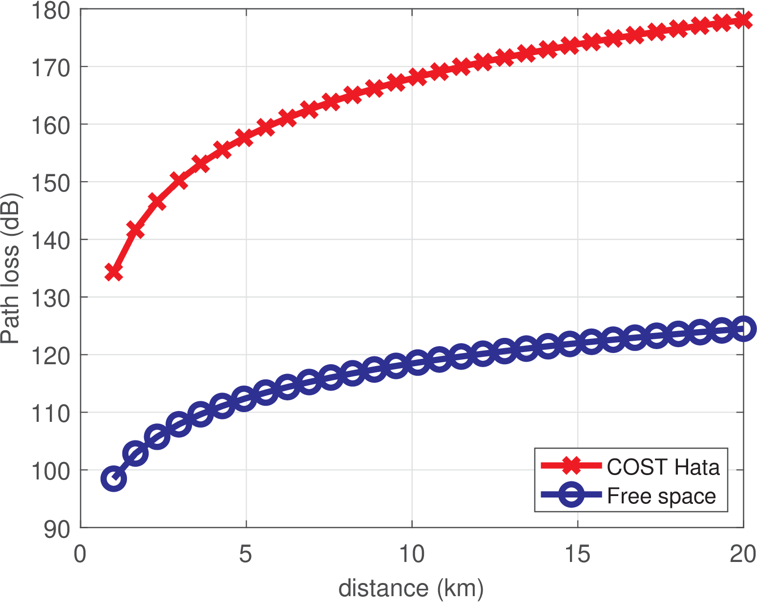
Figure 1.14: Path loss for the free space and COST Hata models, assuming a frequency of 2 GHz.

Figure 1.14 shows the result of executing Listing 1.3. For the adopted frequency of 2 GHz and assuming a distance of 20 km, the COST Hata model predicts a loss of 178.0 dB, while the free space loss (124.5) is 53.5 dB lower.

Example 1.7. GSM coverage distances using COST Hata and free space models. Free space propagation according to Eq. (1.21) provides very optimistic results. In this example, GSM downlink transmission is assumed, with the handset having a standardized receiver sensitivity of $- 102$ dBm. It is assumed a transmitter with power $P_{Tx} = 3$ W (approximately $34.8$ dBm, which is relatively low given that a base station can use e. g. $P_{Tx} = 44.5$ dBm) and antenna gain $G_{Tx} = 6$ dBi. The receiver antenna is limited by the handset size and it is assumed to have gain $G_{Rx} = - 3$ dBi. The feeder cable loss considering both the transmitter and receiver is $L_{cables} = 4$ dB. Using Eq. (1.18), the EIRP is $34.8 + 6 = 40.8$ dBm and Listing 1.4 illustrates how to obtain the maximum distance for the frequencies 900 MHz, 1.8, 2.1 and 2.5 GHz using both the COST Hata and free space models.

For the COST Hata model, it is also assumed the heights of the antennas at the base station and mobile station are 30 and 1.5 m, respectively. The function ak_distanceCost231.m has the path loss as an input parameter and outputs the distance in which this loss is reached.

Listing 1.4: MatlabOctaveCodeSnippets/snip_digi_comm_friis_gsm.m

1c=299792458; %speed of light, approximately 3e8 (meters/second) 
2frequencies=[900 1800 2100 2500]; %frequencies of interest (MHz) 
3Prx=-102; %standardized receiver sensitivity for GSM (dBm) 
4EIRP=40.8; %transmitter equivalent isotropically radiated power (dBm) 
5Grx=-3; %receiver antenna gain (dBi) 
6Lcables=4; %total feeder cable loss, considering both Tx and Rx (dB) 
7Loss=EIRP+Grx-Prx-Lcables; %maximum allowed path loss (dB) 
8Loss_linear=10^(0.1*Loss); %convert from dB to linear scale 
9hbs=53; %effective base station antenna height [m] 
10hms=1.5; %mobile station antenna height [m] 
11category=1; %1: medium-sized city/suburban or 2: metropolitan area 
12for i=1:4 
13    f=frequencies(i); %choose a frequency 
14    d_fs=sqrt(Loss_linear)*c/(4*pi*f*1e6); %find the maximum distance 
15    d_cost=ak_distanceCost231(hbs, hms, f, Loss, category); %COST 
16    disp([num2str(f) ' MHz, FS=' num2str(d_fs/1e3) ' and COST=' ... 
17        num2str(d_cost/1e3) ' km']) %shows both distances 
18end

Omitting the warning messages that indicate some frequencies are outside the range $[1.5, 2]$ GHz for the COST Hata model, the code output indicates the coverage range (in km) for each frequency:

900 MHz, FS=163.4438 and COST=2.4699 km
1800 MHz, FS=81.7219 and COST=1.2298 km
2100 MHz, FS=70.0473 and COST=1.0531 km
2500 MHz, FS=58.8398 and COST=0.88368 km

As expected, the free space (FS) model indicates overly optimistic (large) distances, corresponding to unrealistic coverage. In fact, GSM deployments often limit the cell range to 35 km. The reach predicted by the COST Hata model is more reasonable but, in practice, many aspects influence the actual coverage. Therefore, if possible, a measurement campaign is very useful to tune the model estimation. $□$

The coverage estimation performed in Example 1.7 was relatively simple because a standardized receiver sensitivity (of $- 102$ dBm) was adopted. This allowed the analysis to focus solely on the signal power at the receiver. But, using your intuition, consider a situation in which the noise power at the receiver constantly increases. As discussed in Section 1.7.1, at some point, the communication will be interrupted. An implicit assumption in Example 1.7 is that the actual noise is not stronger than the noise models adopted in the corresponding standard. To properly understand link budgets that account for noise sources, two other important definitions are the noise figure (NF) and noise factor.

1.7.6 Noise factor and noise figure

As discussed in Section 1.5.5, no matter how sophisticated is an electronic device, thermal noise will always affect its performance. The noise factor (F) is used to indicate how much thermal noise is generated by a device, such as an amplifier.

An ideal amplifier simply scales its input as indicated by:

x (t) \to \sqrt{G} \to y (t) = \sqrt{G} x (t)

where the signals $x (t)$ and $y (t)$ are in volts, for example. The voltage gain is denoted by $\sqrt{G}$ because $G$ is reserved to represent the power gain in this section. With $P_{in}$ and $P_{out}$ being the powers of $x (t)$ and $y (t)$ , respectively, one has $P_{out} = G P_{in}$ for the ideal amplifier.

If $x (t) = s (t) + ν (t)$ is composed by a signal of interest $s (t)$ and an additive thermal noise parcel $ν (t)$ , the amplifier scales both, and outputs $y (t) = \sqrt{G} (s (t) + ν (t))$ . It is assumed here that thermal is the only noise present at the device input.

Assuming the powers of $s (t)$ and $ν (t)$ at the amplifier input are $P_{in}^{s}$ and $P_{in}^{t}$ , respectively, the output parcel corresponding to the signal of interest has¹⁴ power $P_{out}^{s} = G P_{in}^{s}$ . For an ideal amplifier that does not generate noise “internally”, the output noise power would simply be $P_{out}^{t} = G P_{in}^{t}$ . However, in practice, this power is modeled with the adoption of a noise factor (F) depicted in Figure 1.15, which allows to write

P_{out}^{t} = G F P_{in}^{t} .

(1.24)

Because $F > 1$ , Eq. (1.24) leads to a value larger than $G P_{in}^{t}$ .

Figure 1.15: The noise factor $F$ depends on the power of the thermal noise generated inside the device, and because $F > 1$ , it increases the input noise power $P_{in}^{t}$ and decreases the SNR at the device output.

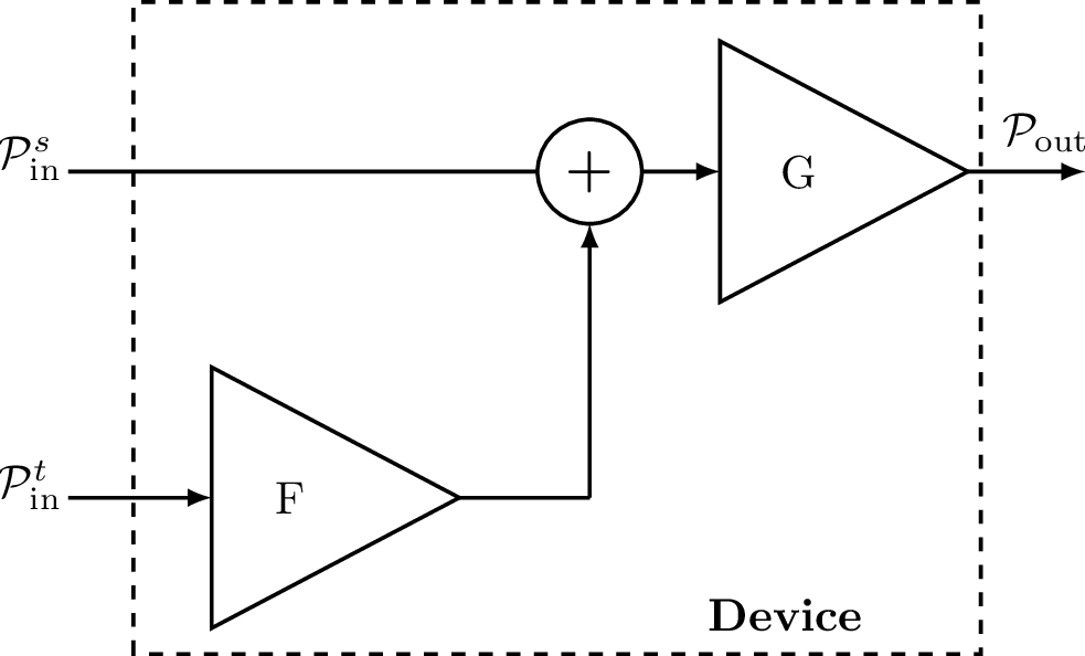
Therefore, a general expression for the output power $P_{out}$ in Figure 1.15 is

P_{out} = P_{out}^{s} + P_{out}^{t} = G P_{in}^{s} + G F P_{in}^{t}

(1.25)

and the SNR at the output can be conveniently written as

{SNR}_{out} = \frac{G P_{in}^{s}}{P_{out}^{t}} = \frac{G P_{in}^{s}}{G P_{in}^{t} F} = \frac{P_{in}^{s}}{P_{in}^{t} F},

(1.26)

such that

F = \frac{{SNR}_{in}}{{SNR}_{out}} .

(1.27)

Eq. (1.27) indicates that, for the adopted model, F is the degradation of SNR caused by a device such as a radio receiver or an amplifier.

A related concept is the noise figure (NF), which is simply the noise factor F converted to dB:

NF = 10 {log}_{10} (F) .

(1.28)

From Eq. (1.28) and Eq. (1.27), one obtains:

{SNR}_{out} = {SNR}_{in} - NF .

(1.29)

The NF represents a decrease in SNR and this can be made equivalent to adding thermal noise at a given temperature.

Note that an ideal amplifier would have $NF = 0$ dB. However, practical circuits have $F > 1$ and, consequently, $NF > 0$ . For example, the NF for the analog front end of modern receivers is typically in the range from 8 to 10 dB. If a low cost receiver has a $NF = 10$ dB and if the SNR at the receiver input is ${SNR}_{in} = 40$ dB, then ${SNR}_{out} = 40 - 10 = 30$ dB at its output. In a link budget, NF can be seen as a loss parcel.

Example 1.8. Using the noise figure for a single amplifier. An amplifier has $G = 6$ and $F = 3$ . According to the notation, the parcels that compose the input signal $x (t)$ have the following powers (all in nW): $P_{in}^{t} = 2$ and $P_{in}^{s} = 100$ , such that $P_{in} = P_{in}^{s} + P_{in}^{t} = 100 + 2 = 102$ . The input SNR is ${SNR}_{in} = 10 {log}_{10} (P_{in}^{s} ∕ P_{in}^{t}) = 10 {log}_{10} (100 ∕ 2) \approx 16.99$ dB.

At the output, the output noise power is $P_{out}^{t} = G F P_{in}^{t} = 6 \times 3 \times 2 = 36,$ which accounts for the amplified $G P_{in}^{t} = 12$ nW plus 24 nW added “internally” by the device. The following diagram summarizes the total noise powers:

P_{in}^{t} = 2 \to G = 6,F = 3 \to P_{out}^{t} = 36 .

The output parcel corresponding to the signal of interest has power $P_{out}^{s} = G P_{in}^{s} = 6 \times 100 = 600$ . Hence, the output SNR is ${SNR}_{out} = 10 {log}_{10} (P_{out}^{s} ∕ P_{out}^{t}) = 10 {log}_{10} (600 ∕ 36) \approx 12.22$ dB.

This result can be obtained by calculating $NF = 10 {log}_{10} 3 \approx 4.77$ and, from Eq. (1.29):

{SNR}_{out} = {SNR}_{in} - NF \approx 16.99 - 4.77 = 12.22,

which is a convenient way to estimate SNRs when calculating a link budget. $□$

One can rewrite Eq. (1.29) as follows. The input SNR is ${SNR}_{in} = P_{in}^{s} - P_{in}^{t}$ (with both power values in dBm). Assuming a white noise unilateral PSD $N_{0}$ in dBm/Hz and a given receiver bandwidth BW in Hz, the noise power (in dBm) is $P_{in}^{t} = N_{0} + 10 {log}_{10} (BW)$ . Hence, Eq. (1.29) can be written as

{SNR}_{out} = P_{in}^{s} - N_{0} - 10 {log}_{10} (BW) - NF .

(1.30)

Example 1.9. Sensitivity of a GSM receiver analog front end. Assume the analog front end (AFE) of a GSM receiver must be designed¹⁵ taking into account that the sensitivity is $S = - 102$ dBm. For GSM using the GMSK modulation and channels with $BW = 200$ kHz, a common target for minimum SNR in 9 dB. It should also be assumed a white unilateral noise PSD with $N_{0} = - 174$ dBm/Hz. This PSD leads to a noise power of

P_{in}^{t} = N_{0} + 10 {log}_{10} (BW) = - 174 + 10 {log}_{10} (200 \times 1 0^{3}) \approx - 121 (in dBm) .

Given the SNR at the AFE output should be ${SNR}_{out} \geq 9$ dB, one can use Eq. (1.30) to require

\begin{array}{l} {SNR}_{out} & \geq 9 \\ P_{in}^{s} - N_{0} - 10 {log}_{10} (BW) - NF & \geq 9 \\ P_{in}^{s} + 121 - NF & \geq 9 \\ NF & \leq P_{in}^{s} + 112 . \end{array}

Assuming, that $P_{in}^{s} = S = - 102$ dBm, the noise figure should be $NF \leq 10$ dB.

Taking three representative examples of NF for a handset AFE: 3 dB (excellent), 5 dB (good), 8 dB (bad), the link margins would be 7, 5 and 2 dB, respectively. $□$

1.7.7 Advanced: Noise figure for a cascade of devices

Different models can be used when considering a cascade of devices or a cascade of components that compose a device, such as filter, mixer and amplifier composing a radio receiver. Figure 1.16 presents a widely used model when a device consists of a cascade of individual components and input thermal noise power $P_{in}^{t}$ is added only at the first stage.¹⁶

Figure 1.16: Model for a cascade of $N$ components with distinct gains and noise factors.

Figure 1.16 leads to an elegant equivalent model for a cascade of $N$ components or devices. In this case, the overall NF of the cascade is given by the Friis formula for noise factor:

F_{cascade} = F_{1} + \frac{F_{2} - 1}{G_{1}} + \frac{F_{3} - 1}{G_{1} G_{2}} + \dots + \frac{F_{N} - 1}{G_{1} G_{2} \dots G_{N - 1}},

(1.31)

where $F_{i}$ and $G_{i}$ are the noise factor and power gain of the $i$ -th stage, respectively, both in linear scale. Therefore, the $N$ amplifiers can be represented by a single stage with noise factor $F_{cascade}$ and gain $G_{cascade} = G_{1} G_{2} \dots G_{N}$ . Listing 1.5 shows an implementation of Eq. (1.31) in Matlab/Octave.

Listing 1.5: Code/MatlabOctaveFunctions/ak_friisCascadeNoiseFactor

1function [Fcascade, Gcascade]=ak_friisCascadeNoiseFactor(F, G) 
2Fcascade = F(1); Gcascade = G(1); %initialization 
3for i=2:length(F) %take in account all stages 
4    Fcascade = Fcascade + (F(i)-1)/Gcascade; %From Friis equation 
5    Gcascade = Gcascade*G(i); %update for next iteration 
6end

Some examples of using Eq. (1.31) are discussed in the sequel.

Example 1.10. Usage of Friis formula for noise factor. Assume $P_{in}^{t} = 2$ and $P_{in}^{s} = 100$ , all in nW, and a cascade of two amplifiers with $G_{1} = 200, F_{1} = 3$ and $G_{2} = 20, F_{2} = 4$ . Listing 1.6 illustrates how to calculate performance indicators for the cascade according to Figure 1.16.

Listing 1.6: Code/MatlabOctaveCodeSnippets/snip_digi_comm_noiseFigureSimpleExample

1G=[200 20]; F=[3 4]; %gains and noise factors (linear scale) 
2%G=[20 200]; F=[4 3]; %gains and noise factors (alternative order) 
3[Fcascade, Gcascade]=ak_friisCascadeNoiseFactor(F, G) %equivalent 
4Pin_s = 100; %power of signal of interest at input 
5Pin_t = 2; %input thermal noise power 
6Pout_s = Pin_s * Gcascade %power of signal of interest at output 
7Pout_t = Gcascade * Fcascade * Pin_t %noise power by cascade 
8Gcascade_dB = 10*log10(Gcascade) 
9NFcascade = 10*log10(Fcascade) 
10SNRin_dB = 10*log10(Pin_s/Pin_t) 
11SNRout_dB = SNRin_dB - NFcascade

Execution of Listing 1.6 informs that ${NF}_{cascade} = 4.79$ dB, the cascaded gain is 36.02 dB the output noise power is $P_{out}^{t} = 24, 120$ nW. The SNR values at the input and output are approximately 16.99 and 12.20 dB, respectively.

The reader is invited to check that by inverting the order of the amplifiers (using the second line of Listing 1.6 instead of the first), the performance is significantly modified: the output SNR in this case is only 10.86 dB. In fact, due to Eq. (1.31), the first device should have a large gain to decrease the impact of the noise factor in subsequent stages. $□$

Example 1.11. Noise figure of a microwave receiver. Assume the receiver of Figure 1.17 (that is a simplified version of Figure 1.12) with NF and gain for each stage listed in Table 1.3. Listing 1.7 shows how to evaluate the cascaded stages.

Figure 1.17: Example of a microwave receiver.

Table 1.3: NF and gain for each stage in Figure 1.12.


Block	Gain (dB)	NF (dB)


Preselector filter	-0.5	0.5

Low noise amplifier (LNA)	25	3

Intermediate frequency (IF) image reject filter	-0.8	0.8

Mixer	-7	7

IF VGA (amplifier)	30	5.5

Listing 1.7: Code/MatlabOctaveCodeSnippets/snip_digi_comm_noiseFigure

1GdB=[-0.5, 25, -0.8, -7, 30]; %gains in dB 
2NF=[0.5, 3, 0.8, 7, 5.5]; %noise figure (always in dB) 
3G=10.^(0.1*GdB); %gains in linear scale 
4F=10.^(0.1*NF); %noise factor (always in linear scale) 
5[Fcascade, Gcascade]=ak_friisCascadeNoiseFactor(F, G); %Friis equ. 
6GcascadedB = 10*log10(Gcascade) %convert back to dB 
7NFcascade = 10*log10(Fcascade) %convert to NF (in dB)

Listing 1.7 informs that ${NF}_{cascade} = 3.64$ dB and the cascaded gain is 46.7 dB in this case.

As suggested by careful inspection of Eq. (1.31), using an amplifier with a large gain in the first stage decreases the impact of the noise added by subsequent stages. This motivates the nomenclature LNA for a good first amplifier in a receive chain. For the given example, ${NF}_{cascade} = 3.5$ dB when considering only the first two stages. Due to the gain of the LNA, the three remaining stages increase ${NF}_{cascade}$ by only $3.64 - 3.5 = 0.14$ dB. $□$

Example 1.12. Using NF with both PSD and absolute power values. This example aims at illustrating how the NF (and gains) can be used with both PSD and absolute power values given that the thermal noise has a flat PSD over the bandwidth BW of interest. For example, the NF can be used to calculate the PSD noise level at the output of a device given that the bandwidth BW will cancel out in some expressions. This can be seen by normalizing both sides of Eq. (1.24) by BW, which leads to

\frac{1}{BW} P_{out}^{t} = \frac{1}{BW} G F P_{in}^{t} \to S_{out}^{t} (f) = G F S_{in}^{t} (f),

where $S_{in}^{t} (f)$ and $S_{out}^{t} (f)$ are the constant PSD values of the thermal noise at input and output, respectively, over BW.

Listing 1.8 provides a numerical example where NF is used to obtain the output noise PSD. In this case, the input signal of interest also has a flat PSD with power $P_{in}^{s} = - 60$ dBm and the input thermal noise has a white PSD with level $N_{0} = - 174$ dBm/Hz. The two amplifiers have gains of 30 and 20 dB, with NF of 2 and 5 dB, respectively.

Listing 1.8: Code/MatlabOctaveCodeSnippets/snip_digi_comm_noiseFigureWithPSD

1GdB=[30 20]; %gains in dB 
2NF=[2 5]; %noise figures (NFs) 
3Pin_s_dBm = -60; %in dBm (absolute power value) 
4PSDin_t_dBmHz = -174; %in dBm/Hz (PSD value) 
5PSDin_t = 10^(0.1*PSDin_t_dBmHz); %in linear scale 
6G=10.^(0.1*GdB); %gains in linear scale 
7F=10.^(0.1*NF); %noise factor (linear scale) 
8[Fcascade, Gcascade]=ak_friisCascadeNoiseFactor(F, G); %equivalent 
9GcascadedB = 10*log10(Gcascade) %gain of cascade in dB 
10NFcascade = 10*log10(Fcascade) %cascade NF 
11Pout_s_dBm = Pin_s_dBm + GcascadedB %in dBm 
12PSDout_t = Gcascade * Fcascade * PSDin_t; %linear scale 
13PSDout_n_dBmHz = 10*log10(PSDout_t) %dBm/Hz, PSD

Running Listing 1.8 calculates the output PSD level as $N_{0} = - 121.99$ dBm/Hz and $P_{out}^{s} = - 60 + 30 + 20 = - 10$ dBm. It can also be observed that the cascade has a NF of approximately 2 dB, i. e., the second amplifier does not impact the total NF significantly due to the relatively high gain of the first amplifier. $□$

1.7.8 Examples of link budgets

Example 1.13. Link budget for downlink satellite transmission.

Listing 1.9 illustrates a link budget for satellite transmission that estimates the carrier-to-noise density ratio $C ∕ N_{0}$ (see Section 1.6.4).

Listing 1.9: MatlabOctaveCodeSnippets/snip_digi_comm_satellite_link_budget.m

1Ptx=16; %transmitter power in dBW 
2Gtx=30; %transmitter antenna gain in dBi 
3EIRP=Ptx+Gtx; %EIRP in dBW 
4distance=37e3; %distance in km 
5freq=12e3; %frequency in MHz (it corresponds to 12 GHz) 
6fspl=32.45+20*log10(distance)+20*log10(freq); %free space loss in dB 
7Grx=35;  %receiver antenna gain in dBi 
8Prx=EIRP-fspl+Grx; %signal power at receiver in dBW 
9noiseTemperature=200 %thermal noise temperature in Kelvin 
10K_boltzmann=1.38e-23; %Boltzmann's constant in Joules/Kelvin 
11N0_rx=10*log10(K_boltzmann*noiseTemperature); %noise PSD in dBW/Hz 
12C_N0=Prx-N0_rx %Carrier-to-noise density ratio in dB*Hz

The output of Listing 1.9 informs $C ∕ N_{0} = 81.2$ dB Hz. $□$

Example 1.14. Link budget for GSM downlink. Listing 1.10 illustrates a GSM link budget that obtains the maximum distance under the specified conditions using the COST Hata model.

Listing 1.10: MatlabOctaveCodeSnippets/snip_digi_comm_gsm_budget.m

1hbs=30; %effective base station antenna height [m] 
2hms=1.5; %mobile station antenna height [m] 
3freq=950; %frequency [MHz] 
4category=1; %1: medium-sized city/suburban or 2: metropolitan area 
5sensitivity=-102; %standardized receiver sensitivity for GSM (dBm) 
6Ptx=45; %transmitter power (dBm) 
7Gtx=10; %transmitter antenna gain (dBi) 
8Grx=-3; %receiver antenna gain (dBi) 
9losses=5; %total feeder cable + connector losses, both Tx and Rx (dB) 
10margin=12; %link margin (dB) 
11EIRP=Ptx+Gtx-losses; %EIRP incorporating losses (dBm) 
12minRxPower=sensitivity+margin-Grx; %minimum power at Rx (dBm) 
13admissibleLoss=EIRP-minRxPower %maximum allowed path loss (dB) 
14dist=ak_distanceCost231(hbs,hms,freq,admissibleLoss,category); % (m)

The output of Listing 1.10 informs that admissibleLoss is 137 dB and the distance (dist) corresponds to approximately 1.95 km. Decreasing the transmitter power Ptx from 45 to 30 dB reduces the reach from 1.95 to 0.73 km. On the other hand, while using Ptx=45, an increase on the base station equivalent antenna height hbs from 30 to 70 m increases this distance to 2.7 km.

It should be noted that GSM handsets typically limit the transmitter power to 2 W, while the base station transmitter power varies in a range from 2 to 300 W. $□$

Example 1.15. Minimum transmitter power for a GSM downlink. This example is slightly distinct from the previous one. As indicated in Listing 1.11, given a specific distance, the goal is to find the required transmitter power Ptx.

Listing 1.11: MatlabOctaveCodeSnippets/snip_digi_comm_gsm_budget2.m

1hbs=30; %effective base station antenna height [m] 
2hms=1.5; %mobile station antenna height [m] 
3freq=900; %frequency [MHz] 
4category=1; %1: medium-sized city/suburban or 2: metropolitan area 
5Gtx=6; %transmitter antenna gain (dBi) 
6Grx=-2; %receiver antenna gain, negative due to body loss (dBi) 
7lossesTx=3; %total feeder cable + connector losses at Tx (dB) 
8margin=12; %link margin to combat fading, etc. (dB) 
9NFrx=6; %receiver noise figure (dB) 
10N0=-174 %thermal (or background) noise floor PSD value (dBm/Hz) 
11BW=25e3; %receiver equivalent noise bandwidth (Hz) 
12distance=1; %distance between antennas (reach)(km) 
13SNRmin=18; %minimum SNR for proper operation at AFE output (dB) 
14%% Calculations: 
15pathLoss=ak_pathLossCost231(hbs,hms,freq,distance,category); % (dB) 
16Pnoise_rx=N0+10*log10(BW); %noise power at receiver (dBm) 
17SNRin=SNRmin+NFrx; %SNR at the receiver AFE input (dB) 
18Prx=SNRin+Pnoise_rx %power of signal of interest at receiver (dBm) 
19requiredEIRP=Prx-Grx+pathLoss+margin; %minimum EIRP (dBm) 
20Ptx=requiredEIRP-Gtx+lossesTx; %obs: EIRP incorporated lossesTx (dBm)

The output of Listing 1.11 informs that Ptx is approximately 31 dBm. Decreasing the frequency to 450 MHz would require only 20.8 dBm (note the COST Hata model is not accurate for such low frequency). $□$

¹² Examples of link budget calculations can be found on the Web. An example of a 802.11 link bugdet with associated margins can be found at [ url5lbu].

¹³ For examples of isotropic radiation and a comprehensive treatment of antennas, see e. g. [ST12], specially Section 4.4 “Antennas in Comm. Systems”, pp. 107.

¹⁴ In this section, all signals are assumed to be uncorrelated, such that the power of a summation of signals is the sum of their individual powers.

¹⁵ See, e. g., the tables for the mobile station (MS) and base transceiver station (BTS) in Section 6.2 at [ url5gss].

¹⁶ An alternative model could consider thermal noise power being added at each stage.