D.10  Applications

This section will briefly discuss some applications of transforms.

Application D.1. Time-localization property of Haar coefficients.

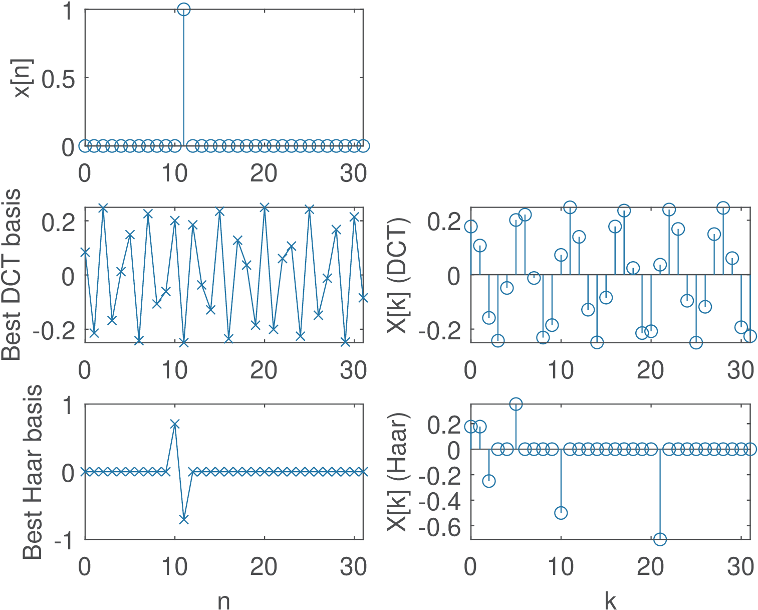
A very simple experiment will help illustrating the time-localization property of Haar functions. Consider the signal to be analyzed in the transform domain is a single impulse $x[n]\; =\; \delta [n\; -n_0],n_0=\; 0,\dots ,31$, which will be represented by a vector $\mathbf{\text{x}}$ will zeroed elements but the one corresponding to the $n_0$ position. The script MatlabOctaveBookExamples/ex_transforms_dcthaar_example.m can be used to observe the behavior of the transforms. Figure D.33 shows the output of the script when the signal is $x[n]\; =\; \delta [n\; -\; 11]$. In this case, many Haar coefficients are zero and the one with largest magnitude ($k\; =\; 21$) has a corresponding basis function (bottom of the left column) that helps to localize the occurrence of the impulse in $x[n]$. In contrast, most DCT coefficients have relatively large values and the basis functions do not help in time-localization. The mentioned script allows to investigate this aspect more deeply. Compare the results of DCT and Haar transforms when the signal is a cosine summed to an impulse.   $\square$

Application D.2. Inverse Laplace transforms with Matlab’s Symbolic Math Toolbox. Keeping in mind that Matlab adopts the unilateral Laplace transform, its Symbolic Math Toolbox can be used to calculate Laplace transforms and their inverses. For example, the unilateral Laplace transform $X(s)\; =\; 1∕s$ of $u(t)$ can be obtained with the commands syms t; laplace(t / t). Similarly, the commands syms w0,t; laplace(sin(w0*t)) indicate that $X(s)\; ={\omega }_0∕(s^2+{\omega }_0^2)$ for $x(t)\; =\; sin({\omega }_{0}t)u(t)$. The following commands illustrate the inverse transform of $X(s)$ given by Eq. (D.54):

1syms s %defines s as a symbolic variable 
2a=1; b=-2; c=-1+j*2; %choose poles and zeros 
3X=(s-a)/((s-b)*(s-c)*(s-conj(c))); %define X(s) 
4ilaplace(X) %Matlab's inverse unilateral Laplace transform

The command pretty (e. g., pretty(ilaplace(X))) can be used to beautify the output, which in this case is - 3/5 exp(-2 t) + 1/5 exp(-t) (3 cos(2 t) + sin(2 t)). Find the inverse Laplace transform for other signals, such as $x(t)\; =\; cos({\omega }_{0}t)u(t)$.    $\square$

Application D.3. ECG transform coding. Because a block transform is completely specified by an invertible matrix $\mathbf{\text{A}}$, going from one domain to another ($\mathbf{\text{x}}$ to $\mathbf{\text{X}}$ or vice-versa) is loss-less, which means there is no loss of information. In many applications, such as image coding, where the goal is to minimize the number of bits to represent an image, it is useful to compress the signal using a lossy algorithm. Transform coding can be a lossy algorithm when it discards or quantizes coefficients in the transform domain. This is effective in many applications because, while all samples in $\mathbf{\text{x}}$ have the same “importance”, in the transform domain $\mathbf{\text{X}}$ the coefficients can be organized according to some hierarchy or rank. In transform coding the most “important” coefficients are quantized more carefully than the unimportant ones.

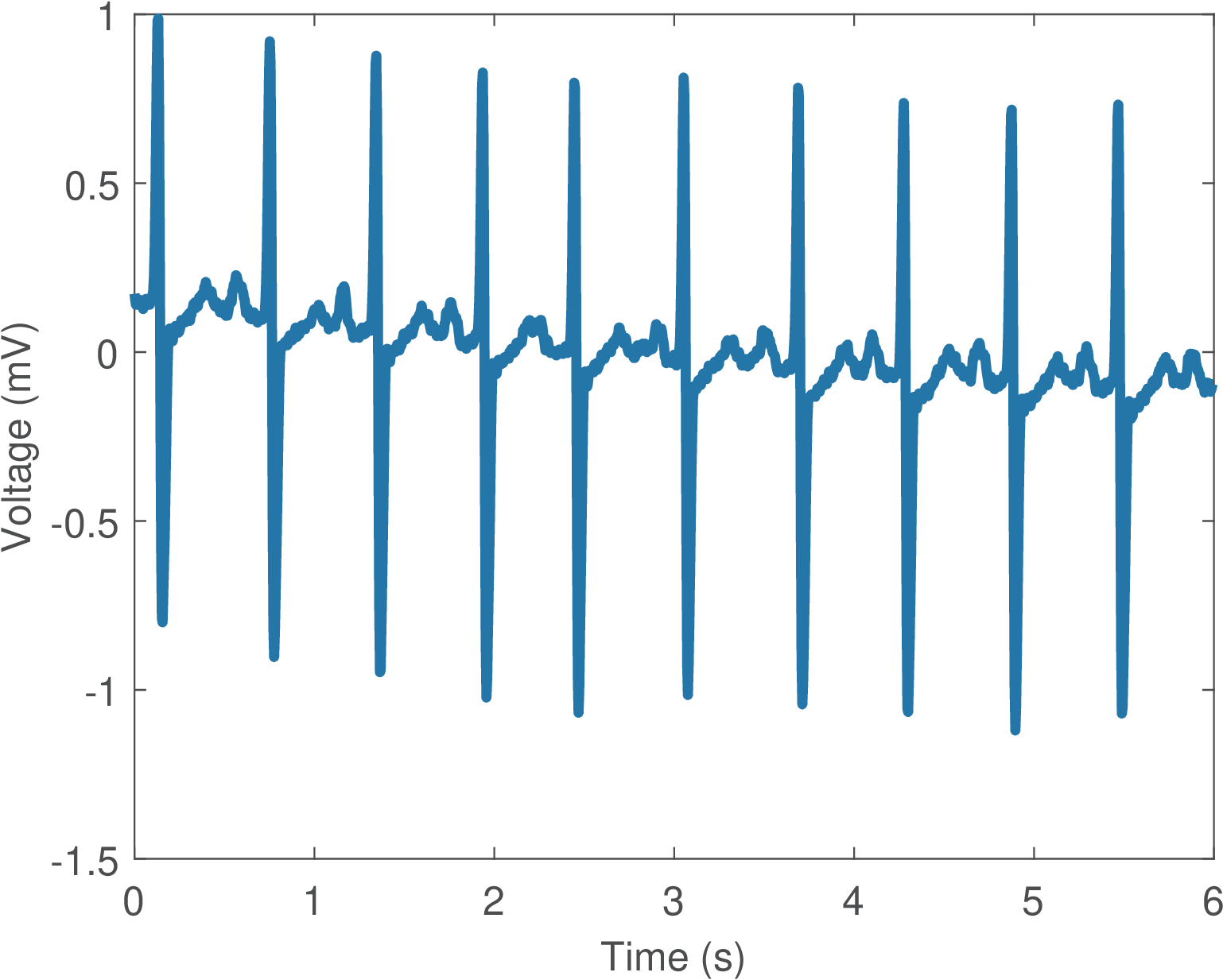
Figure D.34 depicts a segment (first 1,500 samples) of an ECG signal. The ECG data used here is from the MIT-BIH Arrhythmia Database.¹⁸, and Figure D.34 corresponds to the first channel of file 12531_04.dat. The function ak_rddata.m indicates that the DC offset of the ADC chip was calibrated to be zero. It also indicates that the ECG signals were digitized with a sampling frequency $F_s=\; 250$ Hz, 12 bits per sample, and a quantizer with step ${\mathrm{\Delta }}_{\mathrm{\text{AD}}}=\; 1∕400$ mV. The (empirical) signal power is 3.07 mW and, following the conventional quantization model, Eq. (C.20) suggests the quantization noise power was $5.2\; \times \; 10^{-10}$ mW. Hence, the SNR corresponding to the quantization stage alone is approximately 97.7 dB.

A very simple example of a transform coding system is provided as Matlab/Octave code in the companion software (in directory Applications/ECGTransformCoding). The idea is to simply discard the higher-order coefficients in the transform domain. For example, assume that $N$ is the dimension of $\mathbf{\text{x}}$ and $\mathbf{\text{X}}$, which are related by a $N\; \times \; N$ transform matrix $\mathbf{\text{A}}$. In the encoding stage, a discrete-time input signal $x[n]$ is segmented into blocks of dimension $N$, composing a set of $M$ input vectors $\{{\mathbf{\text{x}}}_1,\dots ,{\mathbf{\text{x}}}_M\}$, where $N\; \times \; M$ is the available number of samples of $x[n]$. The coding scheme converts each ${\mathbf{\text{x}}}_i$ into ${\mathbf{\text{X}}}_i=A^H{\mathbf{\text{x}}}_i$ and keeps in a new vector ${\widehat{\mathbf{\text{X}}}}_i$ only the first $K\; \le \; N$ elements of ${\mathbf{\text{X}}}_i$ (the remaining $N\; -\; K$ are discarded). The $M$ vectors ${\widehat{\mathbf{\text{X}}}}_i$ can be concatenated to create an encoded output signal $\widehat{X}[n]$ with $M\; \times \; K$ samples.

In the decoding stage, in order to reconstruct a signal $x\prime [n]$ from $\widehat{X}[n]$ (if there were no losses, $x\prime [n]\; =\; x[n]$), an inverse procedure is adopted. The signal $\widehat{X}[n]$ is blocked into vectors of dimension $K$ and $N\; -\; K$ zero elements are inserted to create vectors $\mathbf{\text{X}}{\prime }_i$ of dimension $N$ (this operation is called zero-padding). Each of these $N$-dimensional vectors is converted to time-domain vectors $\mathbf{\text{x}}{\prime }_i=\mathbf{\text{A}}\mathbf{\text{X}}{\prime }_i$, which are then concatenated to form $x\prime [n]$.

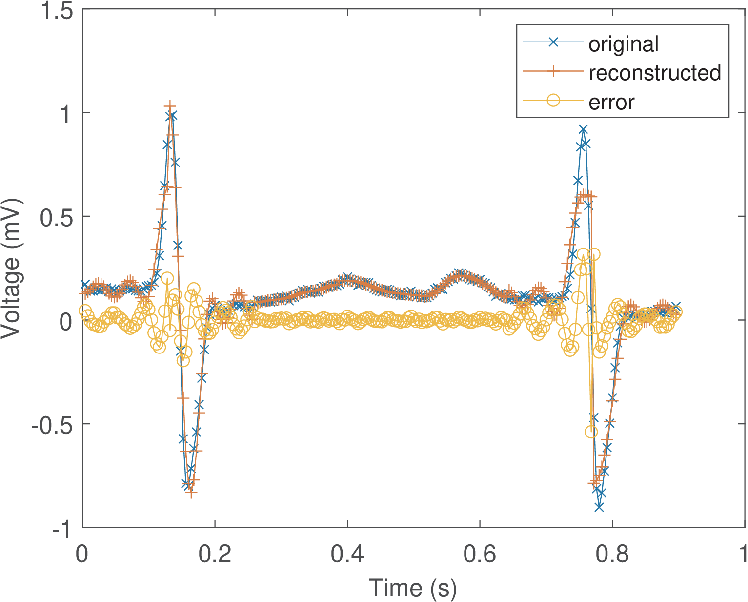
Figure D.35 was obtained using a DCT matrix $\mathbf{\text{A}}$ of $N\; =\; 32$ points and discarding 26 (high-frequency) coefficients. It can be seen that keeping only $K\; =\; 6$ out of 32 coefficients is enough to provide a rough representation of $x[n]$ but the error is significant in high-frequency regions. Note that the DCT operation is performed in blocks of $N\; =\; 32$ samples and Figure D.35 is the result of processing many of these blocks.

In practice, a quantization scheme should be adopted to represent $\widehat{X}[n]$ with a small number of bits per sample. The compression ratio is the number of bits to represent $x[n],n\; =\; 0,\dots ,M\; \times \; N$ divided by the number of bits to represent $\widehat{X}[n],n\; =\; 0,\dots ,M\; \times \; K$. For simplicity, the proposed example does not involve quantization and the compression ratio is evaluated by $N∕K$. This corresponds to assuming that each sample of both $x[n]$ and $\widehat{X}[n]$ is represented with the same number of bits.

Figure D.36 shows the percentage of kept coefficients $K∕N$ in the abscissa and $10{log}_{10}\mathrm{\text{MSE}}$ in the ordinate, where

is the mean-squared error, which is equivalent to the power of the error signal. If $K\; =\; N$ (100% in the abscissa) the system is lossless and $\mathrm{\text{MSE}}=\; 0$ ($-\infty$ in log scale), so the graphs do not show these points. The larger $N$, the better the coding performance but the higher the computational cost.

Assuming $N\; =\; 128$ and $K\; =\; 10$ as indicated in Figure D.36, the abscissa is $K∕N\; =\; 10∕128\; \approx \; 7.81$% and the corresponding error is $\mathrm{\text{MSE}}=\; 1.4824\; \times \; 10^{-8}$ W ($-\; 78.29$ dBW) or, equivalently, $-\; 48.29$ dBm. Given that the signal power was estimated as 3.07 mW ($4.87$ dBm), the ${\mathrm{\text{SNR}}}_{\mathrm{\text{dB}}}\approx \; 4.87\; +\; 48.3\; =\; 53.16$ dB when considering only the distortion incurred by this specific encoding procedure.

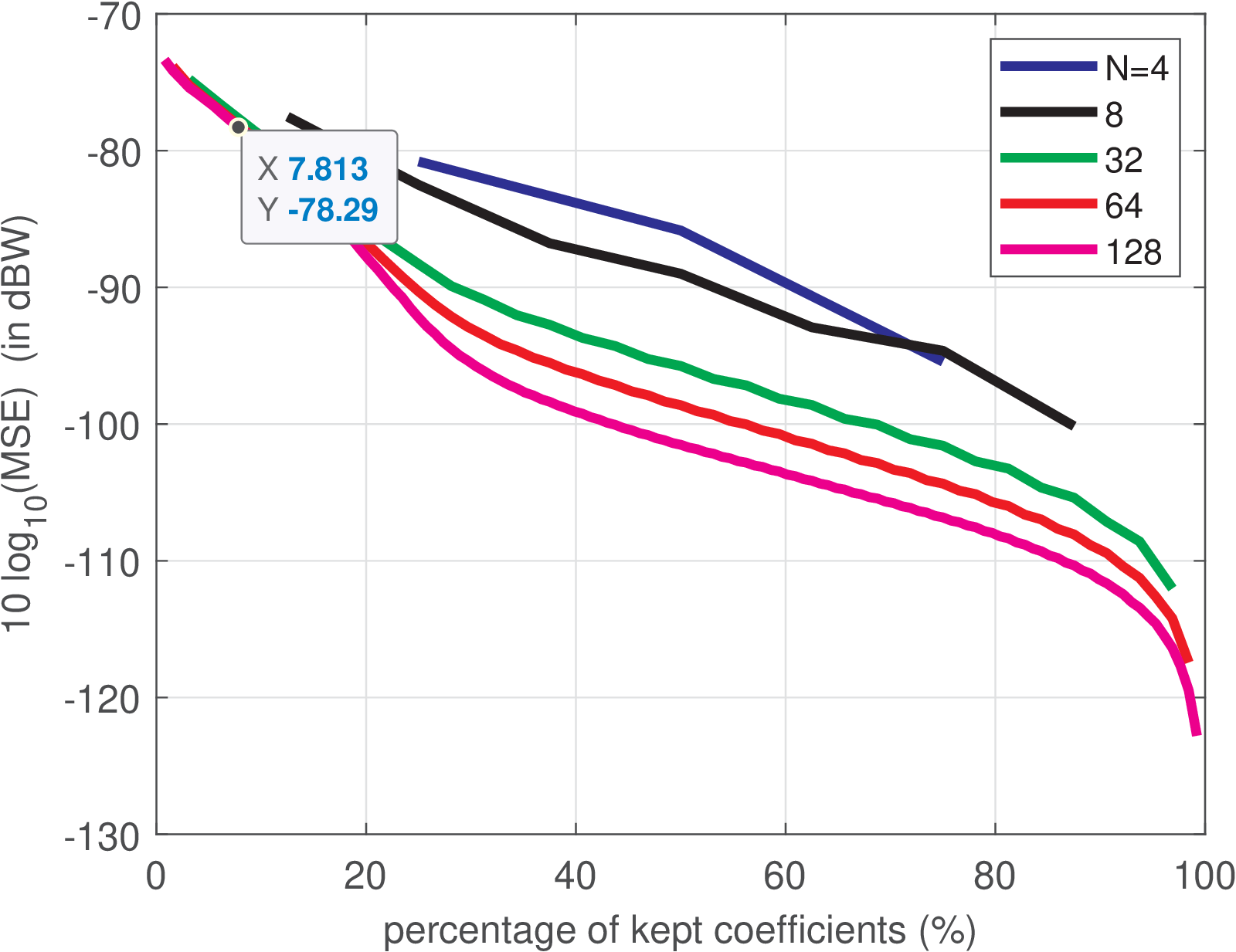
It should be noted that the dataset used is formed by abnormal ECG signals and, eventually, better results could be obtained when using another dataset.

Write an encoder that uses DCT coding to generate files of a relatively small size and a decoder to “decompress” such files and recover an ECG signal (an approximation to the original one). To do that, it is necessary to quantize the DCT coefficients and pack them in a way that the resulting file has a small size. Consider using scalar or vector quantization. The advantage of vector quantization is that you need to store only the index to the codebook entry (codeword) with a vector that will represent the DCT. In case you use a codebook with $2^8=\; 256$ codewords, each entry can be conveniently written as an unsigned char of 8 bits. To design the codebook, besides the Mathwork’s code in the DSP System Toolbox, there are many algorithms such as the K-means with implementations available on the Web.

Another interesting exercise is to apply KLT and other transforms to this problem, trying to get better results than with the DCT.    $\square$

Application D.4. DCT coding of image.

The usefulness of DCT in coding is illustrated by the JPEG image coding standard.¹⁹ Before describing an example, two dimensional transforms are briefly discussed.

Linearly-separable two dimensional (2-D) transforms of a block $\mathbf{\text{x}}$ (e. g., a matrix with pixel values) is obtained by first using the transform along the rows (or columns) and then transforming this result along the columns (or rows). Alternatively, one can use matrix notation: $\mathbf{\text{X}}={\mathbf{\text{A}}}^H\mathbf{\text{x}}{\mathbf{\text{A}}}^{\ast }.$ Because, $\mathbf{\text{A}}$ is real for a DCT, one has

This is equivalent to first calculating $\mathbf{\text{T}}={\mathbf{\text{A}}}^H\mathbf{\text{x}}$: the 1-D DCT transform of each column of $\mathbf{\text{x}}$ is placed in its corresponding column in a temporary matrix $\mathbf{\text{T}}$. Then, each row of $\mathbf{\text{T}}$ is transformed by another 1-D DCT, which could be accomplished by ${\mathbf{\text{A}}}^H{\mathbf{\text{T}}}^T$. This result should be transposed to generate $\mathbf{\text{X}}$. These operations are equivalent to:

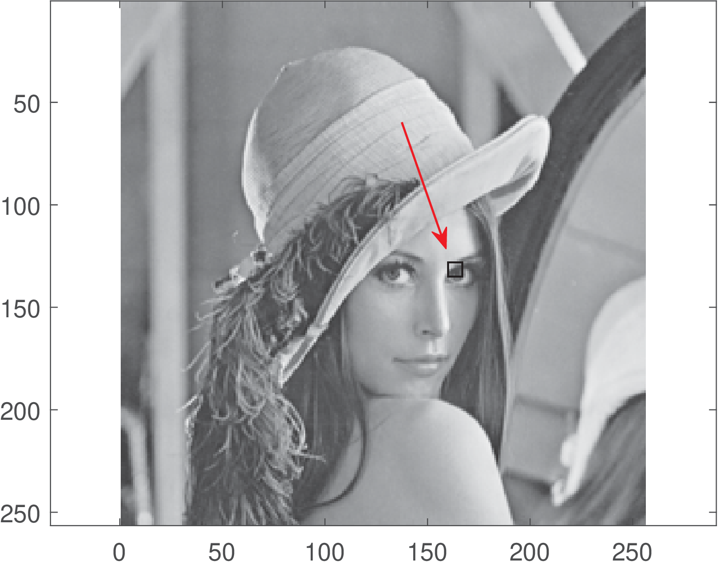
Listing D.5 illustrates the adoption of a 2-D DCT for coding an image block (represented by a matrix).

1%load black & white 256 x 256 pixels of Lenna: 
2fullPath='lenna_bw.gif' %file location 
3  [lenaImage,map]=imread(fullPath); %read file 
4colormap(map); %use the proper color map 
5x1=128; x2=135; y1=160; y2=167; %to take a 8x8 block close to her eye 
6x=lenaImage(x1:x2,y1:y2); %get the region 
7x=double(x); %cast x to be double instead of integer 
8%draw a rectangle to indicate the block: 
9lenaImage(x1,y1:y2)=1; lenaImage(x2,y1:y2)=1; 
10lenaImage(x1:x2,y1)=1; lenaImage(x1:x2,y2)=1; 
11imagesc(lenaImage) %show the image 
12axis equal %correct the aspect ratio 
13%Some calculations to practice: 
14X=octave_dct2(x); %calculate forward DCT 
15x2=octave_idct2(X); %calculate inverse DCT to check 
16numericError = max(x(:)-x2(:)) %any numeric error? 
17Ah=octave_dctmtx(8); %now calculate in an alternative way 
18X2 = Ah*x*transpose(Ah); 
19%X2 = transpose(Ah)*x*Ah; %Note: this would be wrong! 
20numericError2 = max(X(:)-X2(:)) %any numeric error?

Similar to the 1-D ECG coding example in Application D.3, few DCT coefficients can be enough to represent an image. Study the code MatlabOctaveFunctions/ak_dctdemo.m using DCT to represent different images,²⁰ including ones with text. Even better results can be obtained with the wavelet transform, which is used in the JPEG 2000 image coding standard. Write an encoder and decoder that use a transform to compress and decompress an image file.    $\square$

Application D.5. Orthogonality of continuous-time sinusoids over a given interval. In applications such as frequency modulation, it is important to know the conditions in which two cosines with frequencies $f_1$ and $f_2$ and phase $𝜃$, are orthogonal over a given interval $T_{\mathrm{\text{sym}}}$ of interest. Mathematically, this requirement can be expressed as

and, because the phase $𝜃$ is the same for both cosines, this requirement is called “coherent orthogonality”. It can be shown²¹ that this condition is satisfied with integers $m$ and $n$ such that

For example, assume that $T_{\mathrm{\text{sym}}}=\; 0.01$ seconds, $m\; =\; 4$ and $n\; =\; 35$. In this case, $f_1$ and $f_2$ are 1650 and 1850 Hz, respectively. Note that the minimum value of $f_2-f_1$ is $1∕(2T_{\mathrm{\text{sym}}})\; =\; 50$ Hz in this case, which corresponds to choosing $m\; =\; 1$.

As a side note, for “noncoherent orthogonality”, the minimum frequency separation²² is $1∕T_{\mathrm{\text{sym}}}$.    $\square$

Application D.6. Orthogonality of finite duration discrete-time sinusoids. It is also important to evaluate in what conditions a pair of discrete-time sinusoids are orthogonal considering a finite duration interval.

Two discrete-time exponentials $e^{j{\mathrm{\Omega }}_{0}n}$ and $e^{j{\mathrm{\Omega }}_{1}n}$, ${\mathrm{\Omega }}_0\ne {\mathrm{\Omega }}_1$, are always orthogonal when summed over a range $-\infty$ to $\infty$ (see Example D.1), but this is not the case when the summation interval is finite. One way of inspecting what happens when the duration is finite is to reason as following: 1) keep in mind that the sum of the samples of a single sinusoid over a multiple of its fundamental period is zero. 2) Interpreting Example D.3 in discrete-time allows to decompose the inner product for testing orthogonality into a sum of two sinusoids. 3) the inner product is mapped to summations of sinusoids with frequencies equal to ${\mathrm{\Omega }}_0+{\mathrm{\Omega }}_1$ and ${\mathrm{\Omega }}_0-{\mathrm{\Omega }}_1$ and the goal is to find an integer $N$ that is a multiple of both fundamental periods.

One application of this orthogonality principle is the design of a binary transmission, where the two signals are distinguished by their frequencies $f_0$ and $f_1$. This scheme is called frequency shift keying (FSK). We are interested on determining the minimum symbol period that guarantees orthogonality between the two sinusoids. In the context of telecommunications, this minimum period will correspond to the highest symbol rate. The script MatlabOctaveBookExamples/ex_transforms_check_orthogonality.m can be used for studying this question and is repeated below. The sampling frequency is $F_s$ and one should check different pairs of $f_0$ and $f_1$.

1if 1 %choose between two options 
2    f0 = 980;   %frequency of first sinusoid (in telecom, of bit 0) 
3    f1 = 1180;   %frequency of 2nd sinusoid (in telecom, of bit 1) 
4else %another example 
5    f0 = 1650; %1st sinusoid 
6    f1 = 1850; %2nd sinusoid 
7end 
8Fs=9600; %assumed sampling frequency 
9sumSinusoidFrequency = f0+f1; 
10subractSinusoidFrequency = f1-f0; 
11%reduce numbers to rational forms 
12[m,n]=rat(sumSinusoidFrequency/Fs) 
13[p,q]=rat(subractSinusoidFrequency/Fs) 
14Nmin = lcm(n,q) %find the least commom multiple 
15disp(['Minimum common period: ' num2str(Nmin)]) 
16T_duration = Nmin / Fs; %minimum number of samples in seconds 
17%disp(['Maximum symbol rate: ' num2str(1/T_symbolDuration) ' bauds']) 
18%% Check if the product of the two sinusoids is really orthogonal 
19Tsum = 1 / sumSinusoidFrequency; 
20Tsub = 1 / subractSinusoidFrequency; 
21disp('Numbers below should be integers:') 
22T_duration/Tsum 
23T_duration/Tsub 
24Ts=1/Fs; %sampling interval 
25t = 0:Ts:T_duration-Ts; %generate (discrete) time 
26%use sin or cos with arbitrary phase 
27b0 = sin(2*pi*f0*t+4)';  %column vector 
28b1 = sin(2*pi*f1*t)';  %column vector 
29normalizedInnerProduct = sum(b0.*b1) / length(b0) %inner product 
30if (normalizedInnerProduct > 1e-13) 
31    error('not orthogonal! should not happen!'); 
32end

Modify Listing D.6 to use discrete-time sinusoids in radians, not Hz. Assume $N\; =\; 8$ and find a set of $M$ sinusoids that are mutually orthogonal over an interval of eight consecutive samples. What was the maximum value of $M$ that you could find? Now, consider the set of basis functions for a $N$-point DFT and evaluate their orthogonality. Going back to the question about $M$, can it be larger than $N$? Why?   $\square$

Application D.7. Better visualizing the FFT spectrum: Using fftshift to reorganize the spectrum and masking numerical errors. Two improvements of the procedure adopted to obtain Figure D.14 are typically used. The first one is with respect to the range $k\; =\; ⟨N⟩$. Figure D.14 reminds that the definition of an $N$-point DFT assumes $k\; =\; 0,\dots ,N\; -\; 1$. Sometimes it is more convenient to work with ranges that use “negative” frequencies. Typical ranges are $k\; =\; -N∕2,-N∕2\; +\; 1,\dots ,0,1,N∕2\; -\; 1$ when $N$ is even and $-\; (N\; -\; 1)∕2,-(N\; -\; 1)∕2\; +\; 1,\dots ,0,1,(N\; -\; 1)∕2$ when $N$ is odd. In these cases, to represent negative frequencies (or angles in discrete-time processing) the command fftshift can be used. For example, fftshift([0 1 2 3]) returns [2 3 0 1], while fftshift([0 1 2 3 4]) returns [3 4 0 1 2].

The second one aims at eliminating spurious values. Note that, due to numerical errors, the elements of X that should be zero, have small values such as -1.4e-15 - j 3.3e-16, which leads to random angles for $k\ne 1,11$ in Figure D.14. It is a good practice to eliminate these random angles based on a threshold for the magnitude. This post-processing step can be done with a command such as X(abs(X) 1e-12)=0, and is adopted in the Matlab/Octave fft routine.

Figure D.38 benefits from these two improvements and was obtained using Listing D.7.

1k=-N/2:N/2-1; %range with negative k (assume N is even) 
2X(abs(X)<1e-12)=0;%discard small values (numerical errors) 
3X=fftshift(X); %rearrange to represent negative freqs. 
4subplot(211);stem(k,abs(X));subplot(212);stem(k,angle(X));

Note that fftshift does not calculate the FFT but simply reorders the elements in a vector.    $\square$

Application D.8. DTFS analysis of single cosines. Figure D.39 depicts five cosines $x_i[n]\; =\; 10cos({\mathrm{\Omega }}_{i}n)$ with angular frequencies ${\mathrm{\Omega }}_i=\; i2\pi ∕32$ rad, where $i\; =\; 0,1,2,16,31$, and their respective DTFS spectrum calculated with a DFT of $N\; =\; 32$ points and normalized by $N$.

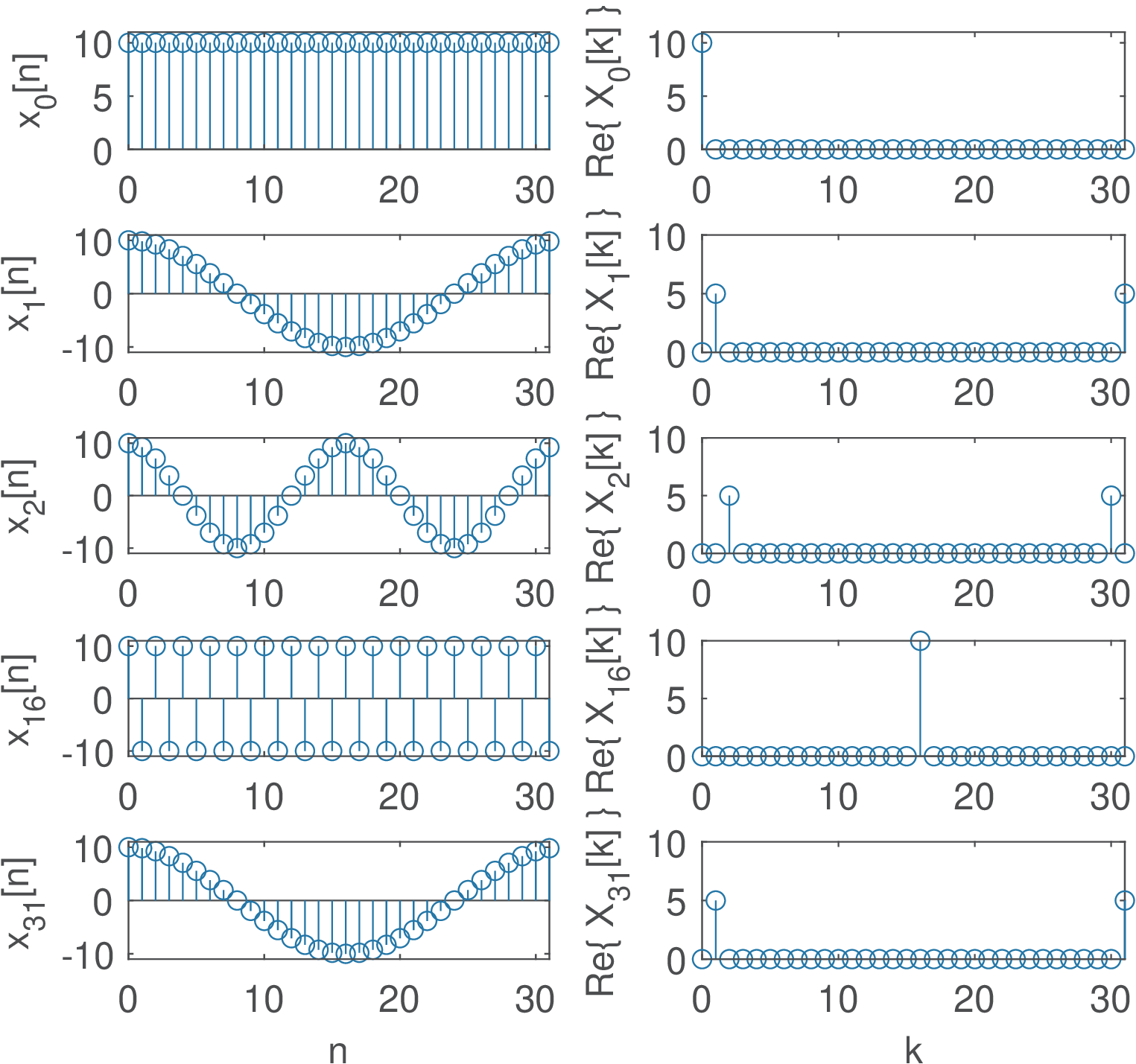
The first $x_0[n]\; =\; 10$ is a DC signal (${\mathrm{\Omega }}_0=\; 0$), the second is $x_1[n]\; =\; 10cos(2\pi ∕32n)$, where ${\mathrm{\Omega }}_1=\frac{2\pi }{32}$ is the fundamental frequency in this DTFS analysis (given that $N\; =\; 32$) and the other three signals are cosines with the following harmonic frequencies: ${\mathrm{\Omega }}_2=\; 2{\mathrm{\Omega }}_1$, ${\mathrm{\Omega }}_{16}=\; 16{\mathrm{\Omega }}_1$ and ${\mathrm{\Omega }}_{31}=\; 31{\mathrm{\Omega }}_1$ rad. Because the cosines are even functions, the imaginary part of their DTFS is zero.

Note in Figure D.39 that the frequency increases up to the $N∕2$-th harmonic ${\mathrm{\Omega }}_{16}=\; 16{\mathrm{\Omega }}_0=\; \pi$. When $N$ is even, the coefficient of $k\; =\; N∕2$ corresponds to $\mathrm{\Omega }=\frac{2\pi }{N}k{|}_{k=N∕2}=\; \pi$. It is important to note that the highest “frequency” of a discrete-time signal is always $\mathrm{\Omega }=\; \pi$ rad.

Another aspect of Figure D.39 is that for $x_0[n]$ and $x_{16}[n]$, corresponding to the angles $\mathrm{\Omega }=\; 0$ and $\mathrm{\Omega }=\; \pi$, the spectra have only one non-zero coefficient $X[k]$, while the other three signals are represented by two coefficients. Figure D.7, for $N\; =\; 4$ and $N\; =\; 6$ can be invoked to help interpreting why the coefficients for angles different than $\mathrm{\Omega }=\; 0$ and $\mathrm{\Omega }=\; \pi$ occur in pairs with Hermitian symmetry (i. e., $X[k]\; =X^{\ast }[-k]$ when $x[n]$ is real). The basis functions for $\mathrm{\Omega }=\; 0$ and $\mathrm{\Omega }=\; \pi$ are real signals while the other angles lead to complex-valued signals. In the analysis of a real signal $x[n]$, using the $k$-th complex basis requires also using the $-\; k$-th basis, such that their imaginary parts can cancel in the synthesis of a real $x[n]$.    $\square$

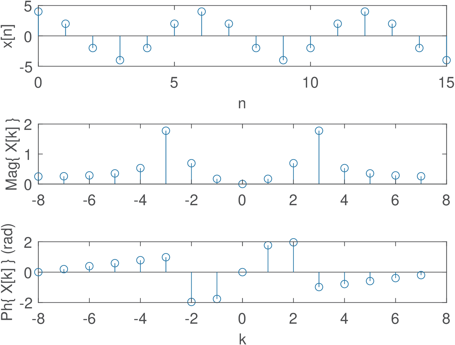
Application D.9. DTFS analysis of a sum of sines and cosines. This example aims at illustrating how the cosines and sines are mapped in the DTFS, especially when two of them have the same frequency. Figure D.40 shows the spectrum of a more complex example obtained with Listing D.8.

1N=32; %number of DFT-points 
2n=0:N-1; %abscissa to generate signal below 
3x=2+3*cos(2*pi*6/32*n)+8*sin(2*pi*12/32*n)-... 
4    + 4*cos(2*pi*7/32*n)+ 6*sin(2*pi*7/32*n); 
5X=fft(x)/N; %calculate DTFS spectrum via DFT 
6X(abs(X)<1e-12)=0; %mask numerical errors

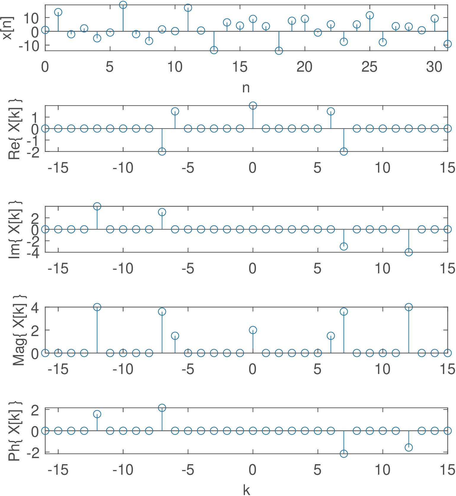
Note in Figure D.40 that the coefficient $X[0]\; =\; 2$ is due to the DC level, $X[6]\; =\; X[-6]\; =\; 1.5$ are due to the cosine $3cos(6(2\pi ∕32)n)$, $X[12]\; =\; -4j$ and $X[-12]\; =\; 4j$ are due to $8sin(12(2\pi ∕32)n)$, $X[7]\; =\; -2\; -\; 3j$ and $X[-7]\; =\; -2\; +\; 3j$ are due to the two parcels of frequency $7(2\pi ∕32)$ with the $-\; 4cos(7(2\pi ∕32)n)$ being represented by the real part ($-\; 2$) and $6sin(7(2\pi ∕32)n)$ represented by the imaginary part ($3j$).   $\square$

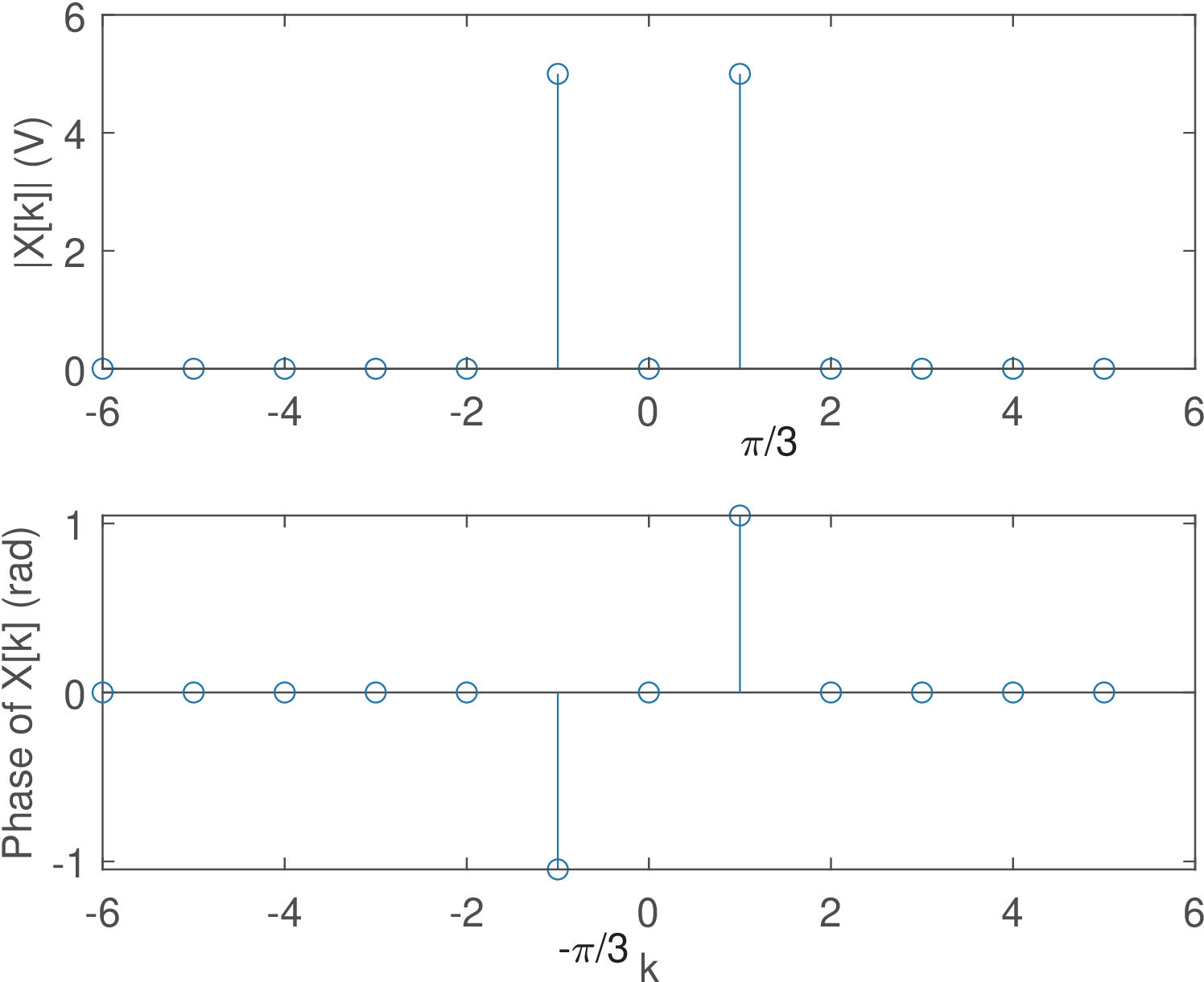
Application D.10. Spurious frequency components: When the number $N$ of DFT points is not a multiple of the signal period. Figure D.41 illustrates the DTFS spectrum of a signal $x[n]\; =\; 4cos((2\pi ∕6)n)$ with period of 6 samples obtained via a 16-point DFT. Note that because 16 is not a multiple of 6, the spectrum has many non-zero spurious components. The coefficients $X[3]\; =\; 0.99\; -\; 1.48j$ and $X[-3]\; =\; 0.99\; +\; 1.48j$, both with magnitude 1.78, are the closest to representing the angle $\pi ∕3\; \approx \; 1.05$ rad. In fact, when using $N\; =\; 16$ points to divide $2\pi$ (see Figure D.7), the angle increment is

which in this case is $\mathrm{\Delta }\mathrm{\Omega }=\; \pi ∕8\; \approx \; 0.39$, and the DFT / DTFS can deal only with the angles $[0,0.39,0.78,1.18,1.57,\dots ,5.89]$ rad. This explains why $X[3]$ and $X[-3]$ are concentrating most of the power $P\; =4^2∕2$. The other coefficients absorb the remaining power that “leaks” due to the imperfect match of the cosine frequency $\pi ∕3$ with the discrete grid of 16 points imposed by the DFT / DFTS.

The creation of spurious components is associated to leakage and the picket-fence effect, which are discussed in Section F.3. This phenomenon is very common when using the FFT to analyze signals that are non-periodic, have infinite duration, etc. In the current case, the spurious components could be avoided by choosing an appropriate number of points for the DFT / DTFS (a multiple of 6). In practice, spurious components due to FFT usage occur most of the times. Even when the original signal is periodic, say $x(t)$ with period $T$, it is typically not guaranteed that $N{T}_s$ is a multiple of $T$, where $N$ is the number of DFT points and $T_s$ the sampling period.

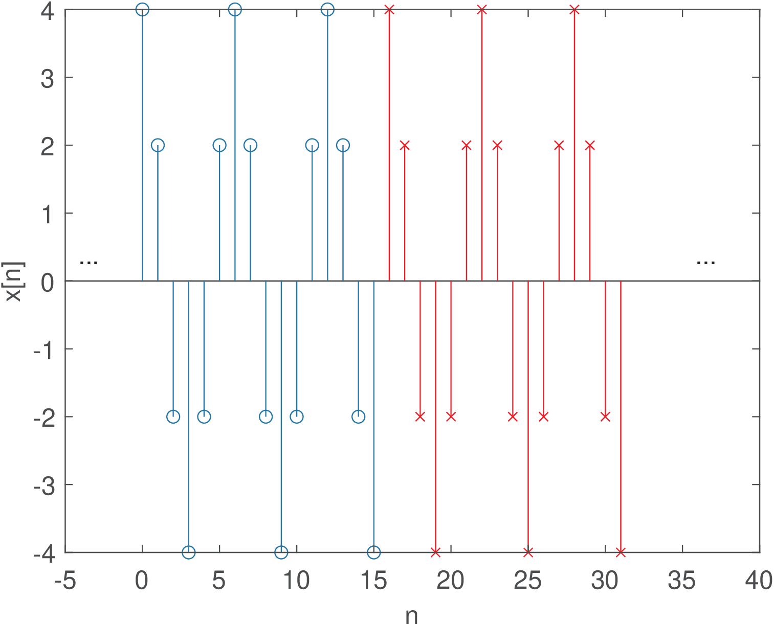
Figure D.42 shows part of the signal obtained by repeating the segment of 16 samples depicted in Figure D.41. This represents the signal “assumed” by the DFT / DTFS. Spurious components appear because, in spite of $x[n]$ having a period of $N\; =\; 6$, an abrupt transition (from $-\; 4$ to 4) occurs in the boundary of the segments of 16 samples. In general, the periodic extension (that is assumed by the FFT when approximating a DTFS) of a signal $x[n]$ not commensurate²³ with its period, leads to discontinuities at the boundaries of the replicas of $x[n]$.    $\square$

Application D.11. DTFS for periodic discrete-time pulses. Assume a periodic train of pulses $x[n]$ with period $N$ and one period described as $x[n]\; =\; 1$ from $n\; =\; 0$ to $N_1-\; 1$ and $x[n]\; =\; 0$ from $N_1$ to $N\; -\; 1$. Its DTFS coefficients are given by

which is the sum of $N_1$ terms of a geometric series with ratio $r\; =e^{-j\frac{2\pi }{N}k}$. Applying Eq. (A.16) leads to

This expression can be simplified by applying Eq. (A.14) to both numerator and denominator:

for $k\; =\; 0,\dots ,N\; -\; 1$ and then periodically repeated in $k$. For $k\; =\; 0$ the expression is undetermined (because of the $0∕0$ fraction) and L’Hospital’s rule leads to $X[0]\; =N_1∕N$.

Listing D.9 obtains the DTFS of the periodic pulses in two distinct ways.

1N=10; N1=5; k=0:N-1; %define durations and k 
2Xk=(1/N)*(sin(k*N1*pi/N)./sin(k*pi/N)) .* ... 
3    exp(-j*k*pi/N*(N1-1)); %obtain DTFS directly 
4Xk(1)=N1/N; %eliminate the NaN (not a number) in Xk(1) 
5%second alternative, via DFT. Generate x[n]: 
6xn=[ones(1,N1) zeros(1,N-N1)] %single period of x[n] 
7Xk2=fft(xn)/N %DTFS via DFT, Xk2 is equal to Xk

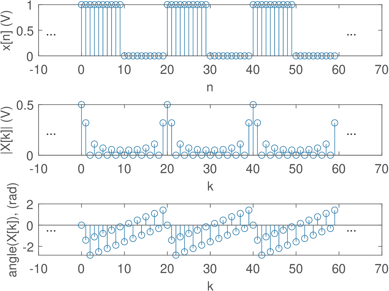
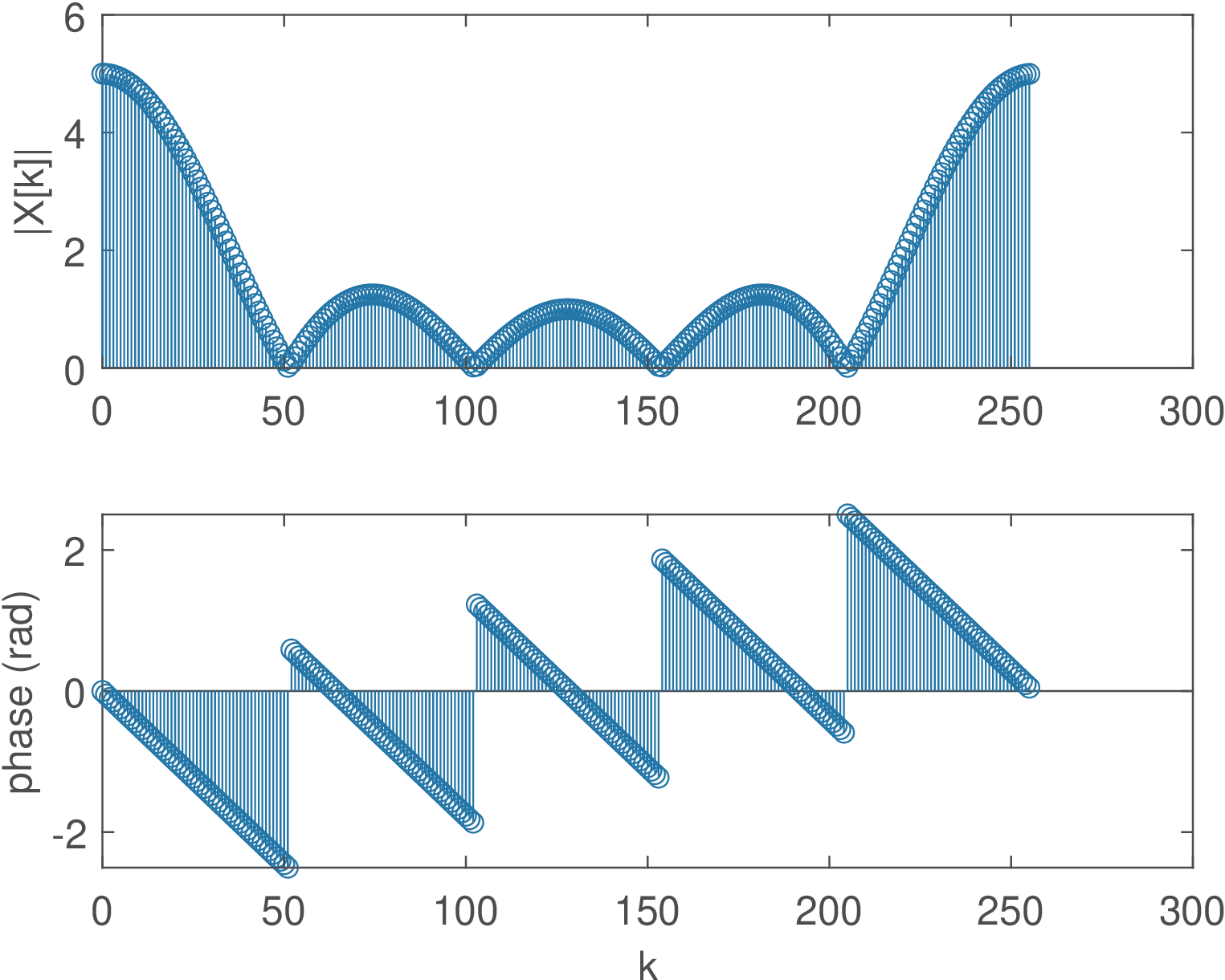
Figure D.43 illustrates the result using $N\; =\; 20$ and $N_1=\; 10$. Note that $|X[k]|$ has the behavior of a sinc function, as expected. The DTFS phase in Figure D.43 c) is the combined effect of the linear phase $e^{-j\frac{k\pi }{N}(N_1-1)}$ and the sign of $sin(k{N}_1\pi ∕N)∕sin(k\pi ∕N)$ in Eq. (D.65). This sign is responsible for Figure D.43 c) not being a linear function of frequency.

(a) $N_1=\; 4$

(b) $N_1=\; 3$

(c) $N_1=\; 2$

(d) $N_1=\; 1$

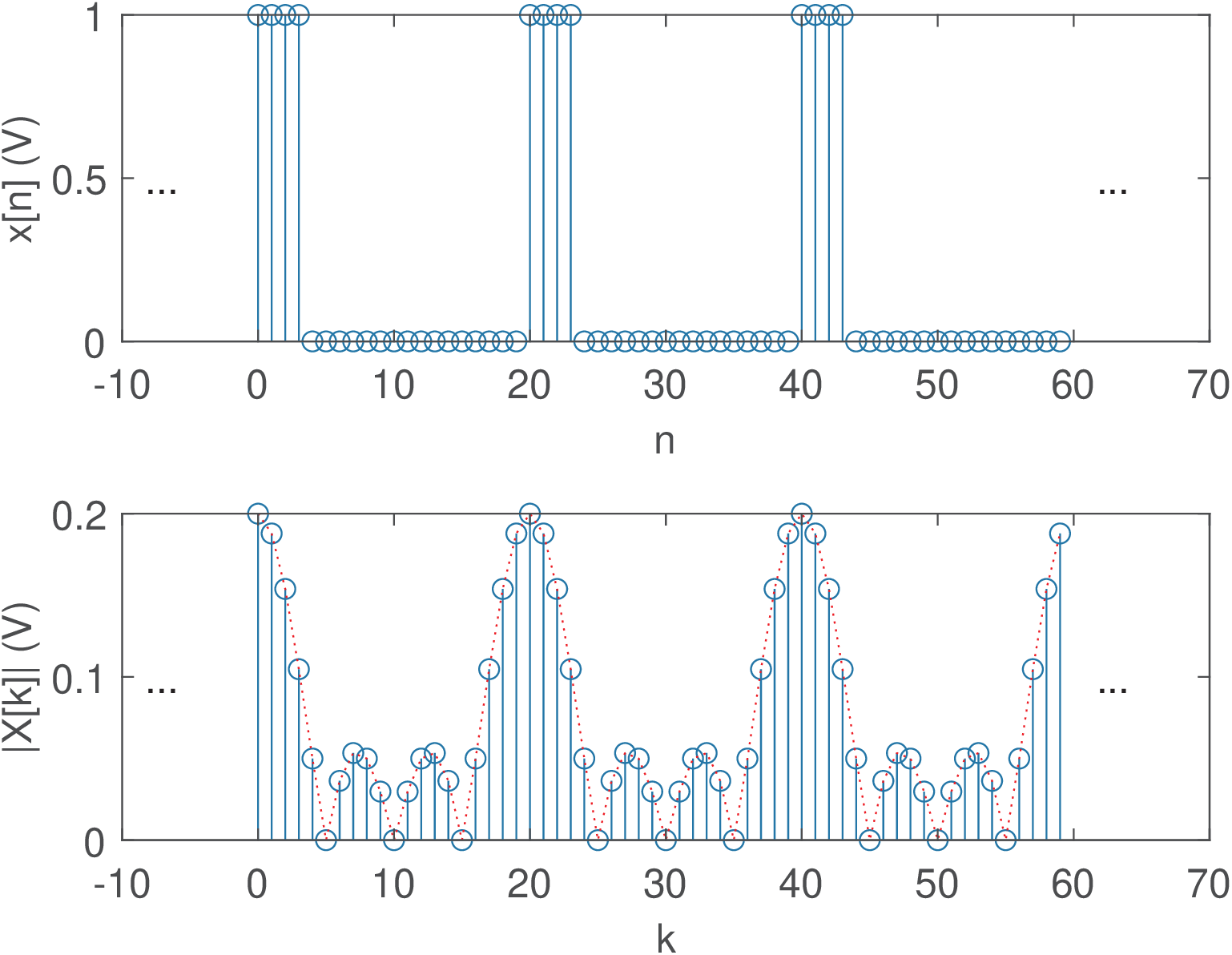
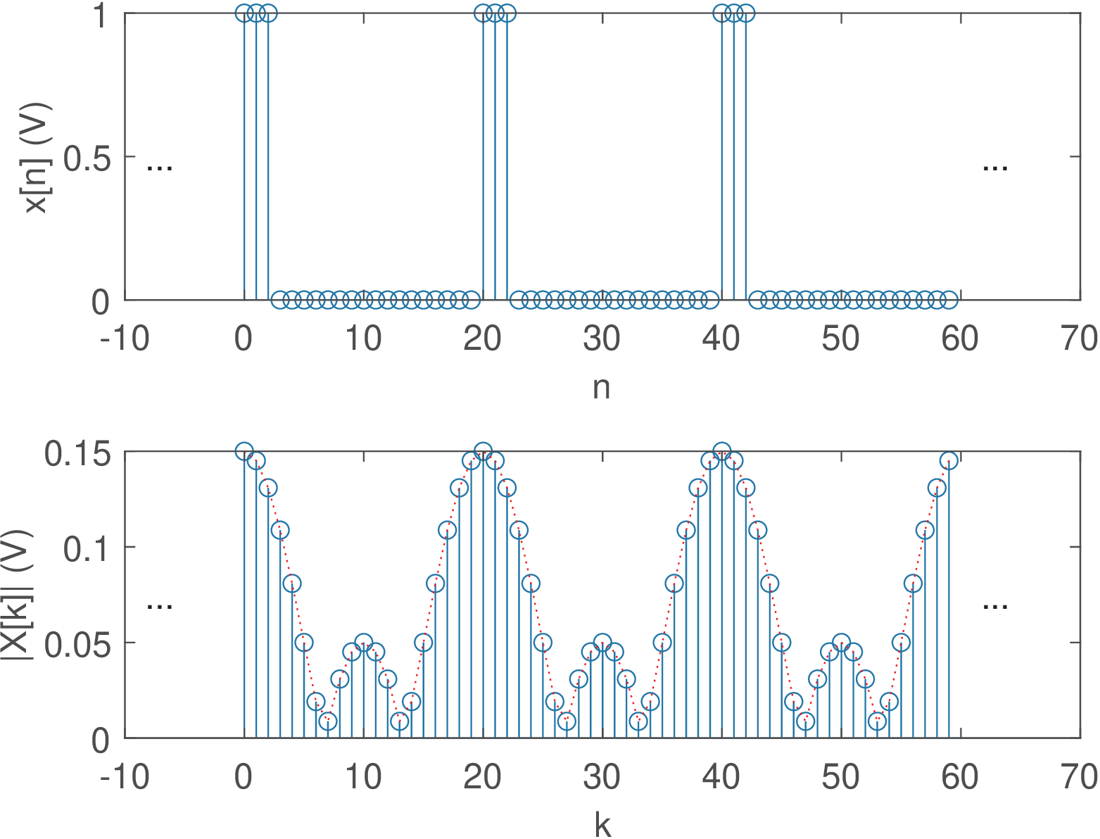
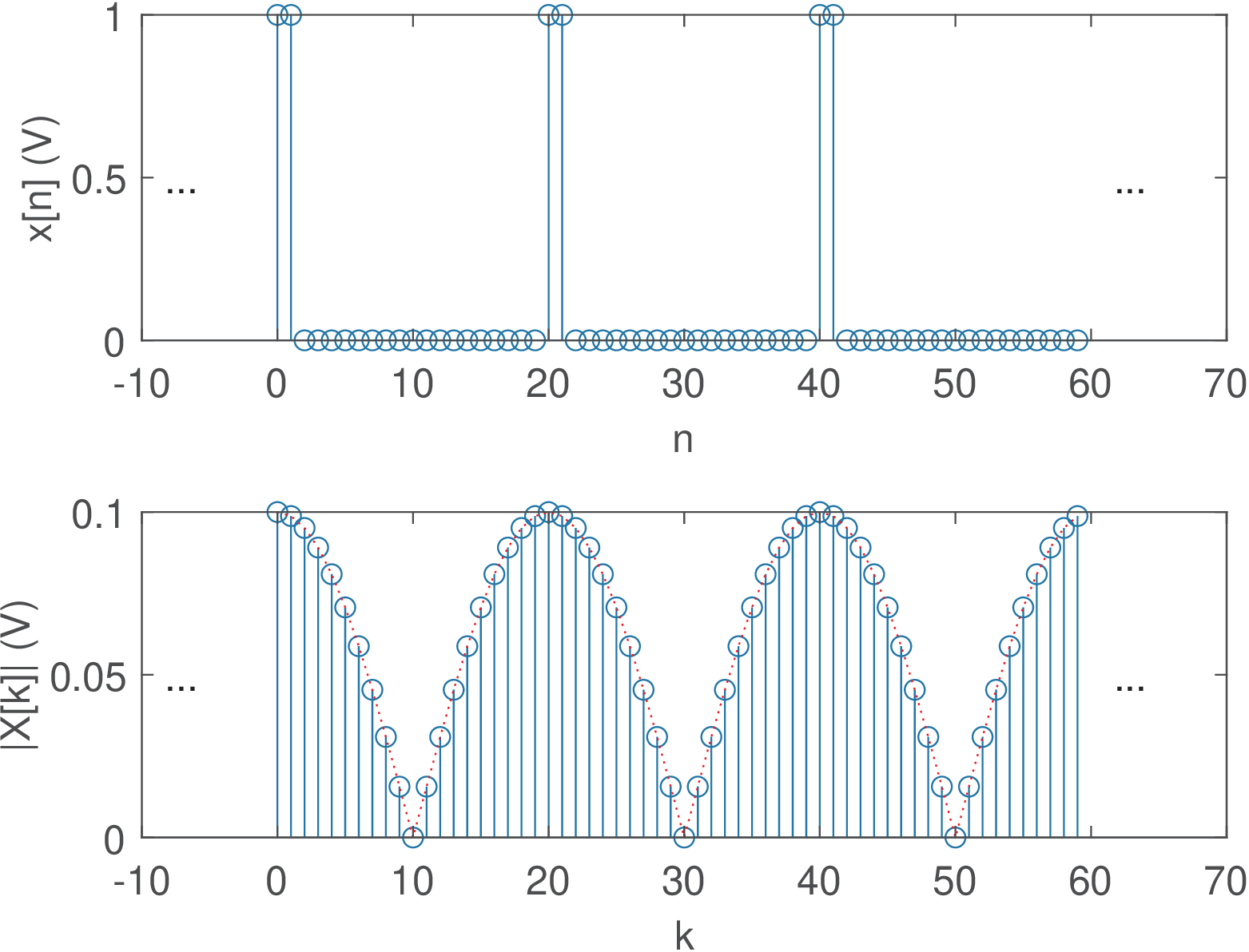
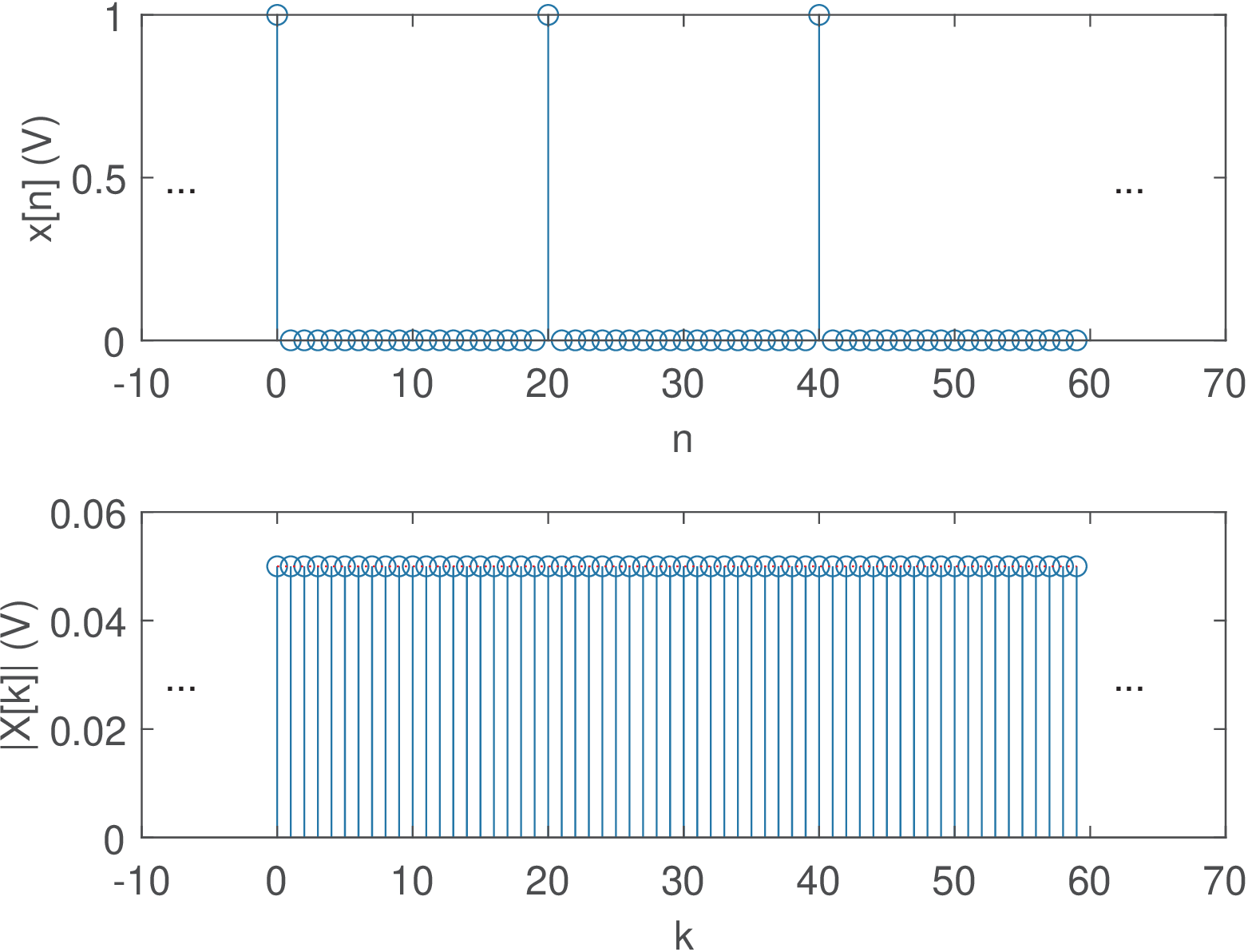
Figure D.44 shows the behavior of the DTFS of $x[n]$ when $N_1$ of Figure D.43 is decreased from $N_1=\; 4$ to 1 Note the duality between time and frequency: as the pulse duty cycle gets smaller (smaller $N_1$), the spectrum gets wider and with smaller maximum values. When $N_1=\; 1$, then $|X[k]|\; =N_1∕N\; =\; 0.05$. Also, in this case, $N_1$ dictates the number of nulls in the spectrum, while $N$ controls how the unit circle $e^{j\mathrm{\Omega }}$ is sampled by the DFT.   $\square$

Application D.12. Calculating the DTFT of a pulse via the DFT. Following steps similar to the ones that led to Eq. (D.65), the DTFT pair of a pulse is given by

Listing D.10 illustrates how to obtain samples of the DTFT for a pulse with $N_1=\; 5$ non-zero samples using a DFT of $N\; =\; 20$ points.

1N=20; %DFT size 
2N1=5; %num. non-zero samples in the (aperiodic) pulse 
3x=[ones(1,N1) zeros(1,N-N1)]; %signal x[n] 
4N2=512; %num. samples of the DTFT theoretical expression 
5k=0:N2-1; %indices of freq. components 
6wk = k*2*pi/N2; %angular frequencies 
7Xk_fft = fft(x); %use N-point DFT to sample DTFT 
8Xk_theory=(sin(wk*N1/2)./sin(wk/2)).*exp(-j*wk*(N1-1)/2); 
9Xk_theory(1) = N1; %take care of 0/0 (NaN) at k=0 
10subplot(211); stem(2*pi*(0:N-1)/N,abs(Xk_fft)); 
11hold on, plot(wk,abs(Xk_theory),'r'); 
12subplot(212); stem(2*pi*(0:N-1)/N,angle(Xk_fft)); 
13hold on, plot(wk,angle(Xk_theory),'r');

The code plots the DTFT superimposed to the DFT result, as illustrated in Figure D.45.

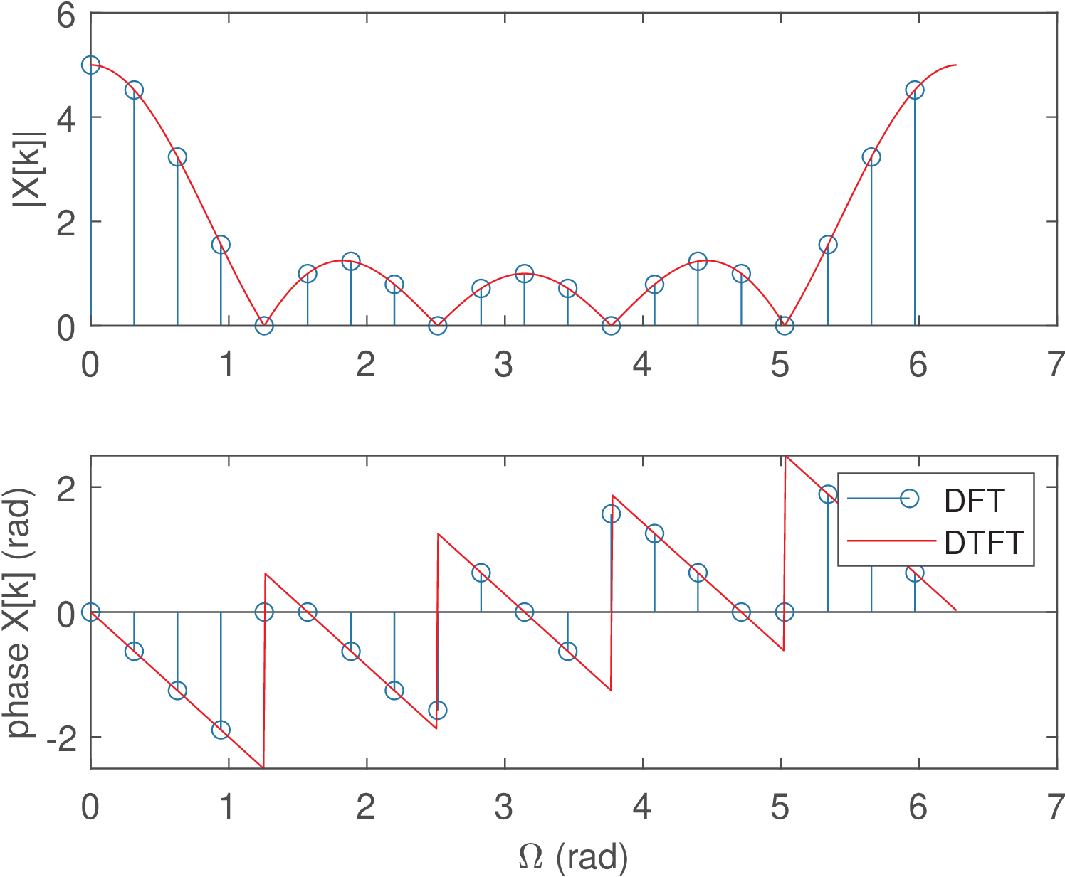
As stated by Eq. (D.35), Figure D.45 pictorially illustrates that the DFT values at the discrete frequencies ${\mathrm{\Omega }}_k=\; k(2\pi ∕N)$ coincide with the DTFT of the aperiodic pulse $x[n]$ calculated at these frequencies using Eq. (D.66).

The DTFT can be calculated in a grid of frequencies with arbitrary resolution by increasing the number $N$ of DFT points. For example, using $N\; =\; 256$ leads to the spectrum in Figure D.46. Note that if x has less than $N$ samples, the command fft(x,N) conveniently extends its duration with zero-padding.    $\square$

Application D.13. Calculating the DTFT using Matlab/Octave’s freqz. When $N$ is relatively large, it is more convenient to use plot instead of stem (as in Figure C.19), in spite of $X[k]$ being discrete. This is also convenient when $X[k]$ is used to represent values of $X(e^{j\mathrm{\Omega }})$ as in this example. Matlab/Octave has the command freqz that uses the DFT to calculate the DTFT at a grid of discrete frequencies. Assuming the same vector x of the previous code snippet, the command freqz(x) generates Figure D.47.

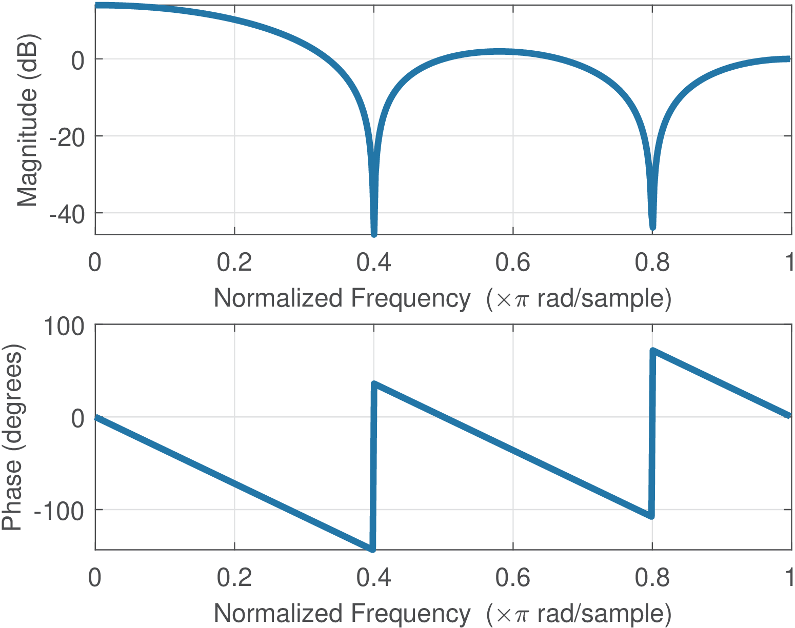
Note that Figure D.46 and Figure D.47 provide the same information in spite of looking quite different. For instance, Figure D.47 is not explicitly showing that the DTFT is being calculated only at a grid of discrete frequencies.

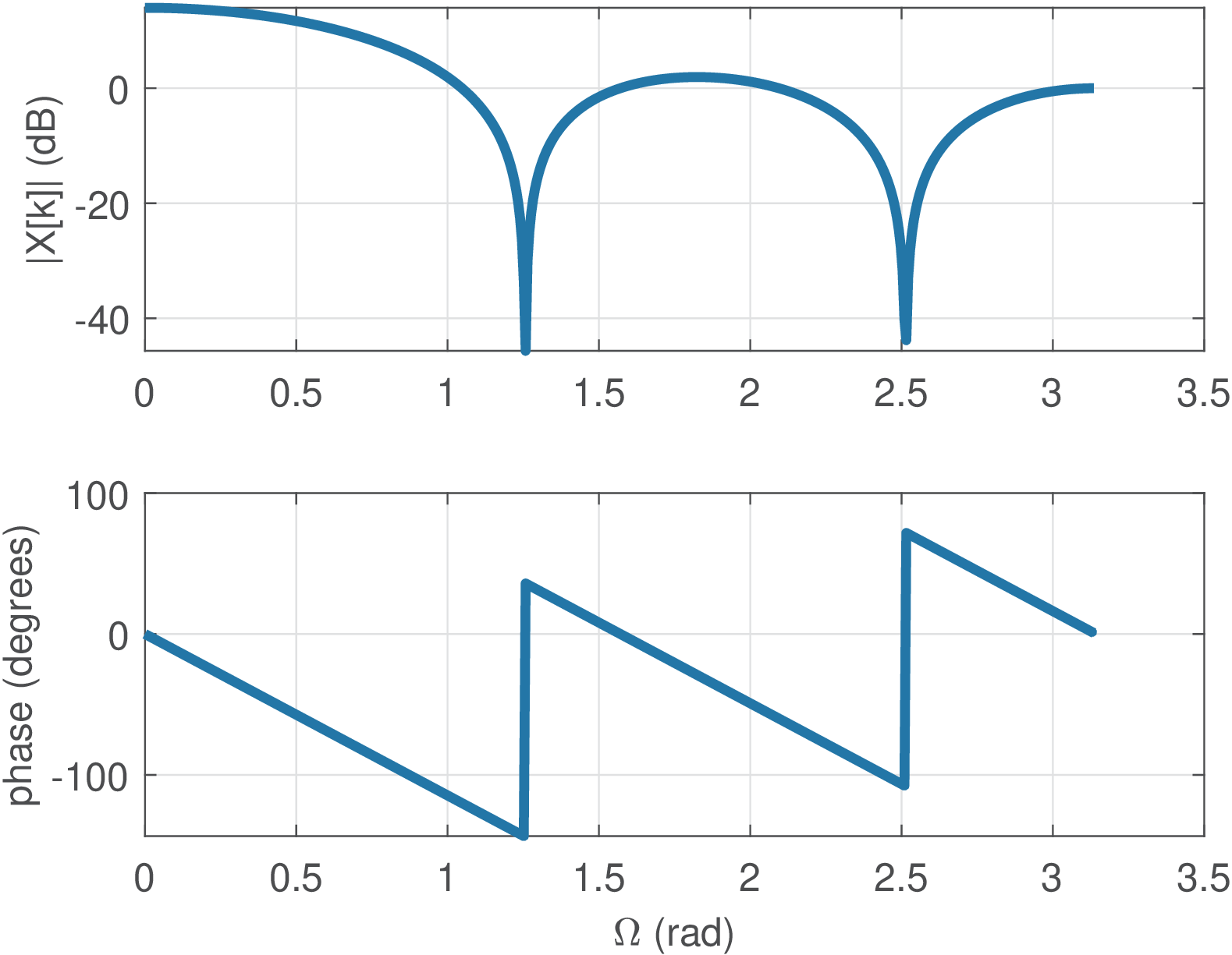
To better understand how freqz works, Listing D.11 mimics freqz and was used to obtain Figure D.48.

1N1=5; %num. non-zero samples in the (aperiodic) pulse 
2x=[ones(1,N1) zeros(1,2)]; %signal x[n] 
3halfN=512; N=2*halfN; %half of the DFT dimension and N 
4k=0:N-1; %indices of freq. components 
5wk = k*2*pi/N; %angular frequencies 
6Xk_fft=fft(x,N);%use 2N-DFT to get N positive freqs. 
7Xk_fft=Xk_fft(1:halfN);%discard negative freqs. 
8wk=(0:halfN-1)*(2*pi/N); %positive freq. grid 
9subplot(211); plot(wk,20*log10(abs(Xk_fft))); %in dB 
10subplot(212); plot(wk,angle(Xk_fft)*180/pi); %in degrees

It can be seen that Figure D.48 is very similar to Figure D.47. The only distinction is that, by default, Matlab/Octave represents the abscissa normalizing $\mathrm{\Omega }$ by $\pi$, such that the maximum frequency is not $\pi$ but 1. It is interesting to note that Matlab/Octave and GNU Radio, for example, indicate $\mathrm{\Omega }$ in rad/sample, while this and other texts assume $\mathrm{\Omega }$ is given in radians ($n$ is dimensionless).   $\square$