A.30  System Properties

It is useful to characterize systems according to well-defined properties. Some of the most important properties are: linearity, time invariance, causality, stability, invertibility and memory. In the next subsections, it is assumed that the inputs $x$, $x_1$ and $x_2$ lead to the outputs $y\; =H\{x\}$, $y_1=H\{x_1\}$ and $y_2=H\{x_2\}$, respectively (note it is not assumed the system $H$ is LTI).

A.30.1  Linearity (additivity and homogeneity)

Linearity is a composition of two properties: additivity and homogeneity. A system (or an operator) is additive if it obeys

which indicates that its output to the sum of two signals $x_1+x_2$ is equal to the sum of the two outputs $y_1$ and $y_2$ obtained independently for $x_1$ and $x_2$, respectively.

If a system is described by the relation $y[n]\; =\; 3x[n]\; +\; 2x[n\; -\; 1]$ it is additive. The proof is as follows. When $x[n]\; =x_1[n]\; +x_2[n]$ one has

On the other hand, a system with $y[n]\; =\; 3{(x[n])}^2$ is not linear because

A system is homogeneous in case

where $\alpha \; \in \; ℂ$. In this case, if the input is multiplied by $\alpha$, the output is multiplied by the same factor $\alpha$. For example, the system $y[n]\; =\; 3{(x[n])}^2$ does not obey homogeneity because

On the other hand, $y[n]\; =\; 3x[n]\; +\; 2x[n\; -\; 1]$ can be proved to be homogeneous. Because it is also additive, $y[n]\; =\; 3x[n]\; +\; 2x[n\; -\; 1]$ is a linear system.

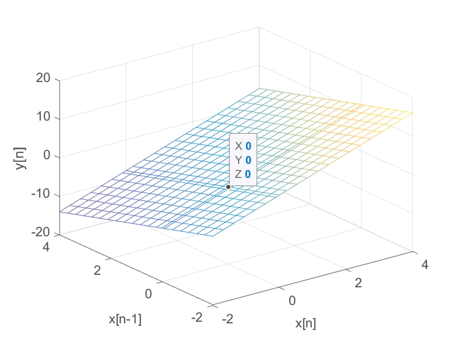
To provide a geometrical description of linearity, Figure A.35 depicts the possible outputs of the system $y[n]\; =\; 3x[n]\; -\; 2x[n\; -\; 1]$ as triples $(x[n],x[n\; -\; 1],y[n])$. The plot shows the output when $x[n]$ and $x[n\; -\; 1]$ are obtained from a grid of 400 Cartesian points in the range $[-2,4]\; \times \; [-2,4]$. It can be seen that, as required for a linear system, the input $(x[n],x[n\; -\; 1])\; =\; (0,0)$ leads to $y[n]\; =\; 0$. In contrast, the system $y[n]\; =\; 3x[n]\; +\; 2x[n\; -\; 1]\; +\; 1$ is not linear (neither additive nor homogeneous). A linear system is required to respond to an all zero input $x[n]\; =\; 0,\forall n$ with an all zero output $y[n]\; =\; 0,\forall n$.

Linearity is also called the principle of superposition and can be written as

A.30.2  Time-invariance (or shift-invariance)

A system is time-invariant in case

or, in the discrete-time case: $y[n\; -n_0]\; =H\{x[n\; -n_0]\}$, which is also called shift-invariant.

Time-invariance is equivalent to having the output delayed (or anticipated) by the same amount that the input was. A valid analogy is to consider that someone has a strict personal routine, which consists in waking-up at 7am, having breakfast at 8am, brushing teeth at 9am and so on. This person would be time-invariant if, in case it wakes-up late, at 10am, it would keep the same routine with a delay of 3 hours: breakfast at 11am, brushing teeth at noon, etc.

A system $y[n]\; =\; nx[n]$ is not time-invariant. To prove it, one can observe that for an input $x[n]\; =\; \delta [n\; -\; 2]$, the output is $y[n]\; =\; 2\delta [n\; -\; 2]$ (because $x[n]\; =\; 0,n\ne 2$). Now, if one delays the input by $n_0=\; 4$, to create a new input $x\prime [n]\; =\; x[n\; -n_0]\; =\; \delta [n\; -\; 6]$ the output is $y[n]\; =\; 6\delta [n\; -\; 6]$, which is different from having the output delayed by the same amount $n_0=\; 4$ and get $y[n]\; =\; 2\delta [n\; -\; 6]$, which should be expected for a time-invariant system.

It is easier to prove that a property is not respected because it suffices to give a single example that violates the property. However, to prove that a system obeys a property, this must be done in a general setting, to prove that it works for all signals. To practice this kind of general proof, let us continue with the system $y[n]\; =\; nx[n]$. The output to $x[n\; -n_0]$ is $(n\; -n_0)x[n\; -n_0]$ while time-invariance would require the output to be $nx[n\; -n_0]$. Before stating a general proof, it is convenient to work out a simple example.

As another example, the system $y(t)\; =\; 3x(t)\; +\; 2x(t\; -\; 1)$ is time-invariant because for $x(t\; -t_0)$ the output is $y(t\; -t_0)\; =\; 3x(t\; -t_0)\; +\; 2x(t\; -\; 1\; -t_0)$.

A.30.3  Memory

A memoryless system has the output at time $t_0$ depending only on the input at time $t_0$. This means that the output of a memoryless system does not depend of any past or future history of the input. For example, in analog filters, the resistor is a component that does not have memory, while the capacitor and inductor have. The current-voltage relation for a resistor is $i(t)\; =\; v(t)∕R$ (memoryless) while for a capacitor it is $i(t)\; =\; Cdv(t)∕dt$, which depends of the variation of $v(t)$ with time.

It is relatively easy to identify memory in the discrete-time domain because it can be related to the actual storage space called “memory” in computing systems. For example, the system $y[n]\; =\sqrt{x[n]}+{exp}^{x[n]}$ is memoryless, while $y[n]\; =\; x[n]\; +\; 2x[n\; -\; 1]\; -\; y[n\; -\; 15]$ has to store one previous value ($x[n\; -\; 1]$) of the input and 15 previous values ($y[n\; -\; 1],y[n\; -\; 2],\dots ,y[n\; -\; 15]$) of the output. As illustrated in Listing E.12, all these values need to be stored in “memory” positions. The storage space for $x[n]$ and $y[n]$ is not accounted, even if in practice they require space. For example, assuming the values are represented as 4-bytes “floats”, the previous system would require $4(1\; +\; 15)\; =\; 64$ bytes of RAM “memory” to store the system memory.

A.30.4  Causality

A system is causal if the output at instant $t_0$ depends only on $x(t),t\; \le t_0$, i. e., does not depend on future values of the input. All physical systems are causal because they cannot react to something that will occur in future.²⁶ It is possible to implement a non-causal system if the signal is processed “off-line”, i. e., the samples are pre-stored and the processing is done without concerns to the real life time. The function filtfilt in Matlab/Octave is an example of non-causal processing that is very useful because can filter the magnitude of a signal without influencing its phase.

The system $y[n]\; =\; x[n\; +\; 1]$ is non-causal because $y[n_0]$ depends on $x[n_0+\; 1]$. On the other hand, the system $y[n]\; =\; x[n\; +\; 1]\; -\; 0.5y[n\; +\; 1]$ is causal because the time index can be rearranged (via a change in variable: $n\prime \; =\; n\; +\; 1$) and the system rewritten as $y[n]\; =\; 2x[n]\; -\; 2y[n\; -\; 1]$. As a general rule to check causality, one can look at the output value $y[n\; +n_{\mathrm{\text{max}}}]$ most advanced in time ($n_{\mathrm{\text{max}}}=\; 1$ in previous example), change variables with $n\prime \; =\; n\; +n_{\mathrm{\text{max}}}$, isolate $y[n]$ and check if it depends on future values of the input. For example, the system $y[n\; -\; 3]\; =\; x[n\; -\; 2]\; +\; y[n\; -\; 4]$ is non-causal. This is clear if it is rewritten as $y[n]\; =\; x[n\; +\; 1]\; +\; y[n\; -\; 1]$.

A.30.5  Invertibility

A system is invertible if the input signal can be uniquely determined from the output. This is similar to the concept of an injective function. For example, $y(t)\; =\; kx(t)$ is invertible because $x(t)\; =\; (1∕k)y(t)$, but $y(t)\; =x^2(t)$ is not. In general, a system $H$ is invertible if it is possible to find another system $H^{-1}$ such that their cascade replicates the input, as illustrated below:

A.30.6  Stability

The output of an unstable system can eventually grow unbounded and go to infinite. This is typically undesirable and suggests the so-called bounded-input, bounded-output (BIBO) stability. A system is BIBO stable if the output is bounded whenever the input is bounded. Note that if the input grows unbounded, then a stable system can have its output converging to infinite. In other words, looking only at the output one cannot state whether or not a system is stable. For example, the system $y(t)\; =\; 10x(t)$ is BIBO stable, but if $x(t)\; \to \infty$, then $y(t)\; \to \infty$. On the other hand, the system $y(t)\; =\; 1∕x(t)$ is not BIBO stable, because the bounded input $x(t)\; =\; 0,\forall t$, leads to $y(t)\; \to \infty$.

A.30.7  Properties of linear and time-invariant (LTI) systems

If an LTI system $H$ is memoryless, its impulse response is non-zero only at $n\; =\; 0$ (or $t\; =\; 0$). In other words, $h[n]\; =\; 0,n\ne 0$. $H$ is causal if and only if (i. e., the output does not effectively start until the impulse $\delta [n]$ is applied at $n\; =\; 0$). If an LTI system $H$ with impulse response $h[n]$ is invertible, the inverse system is also LTI and has an impulse response $h_i[n]$ that obeys $h[n]\ast h_i[n]\; =\; \delta [n]$. To be BIBO stable, the LTI must have the impulse response absolutely summable or integrable, i. e.

depending if the system is discrete or continuous in time, respectively.