A.31  Fixed and Floating-Point Number Representations

Unless specified otherwise, Matlab/Octave uses double precision. For example, the commands clear all;x=3;whos generate the following output:

     Variables in the current scope:
        Attr Name        Size                     Bytes  Class
        ==== ====        ====                     =====  =====
             x           1x1                          8  double
     Total is 1 element using 8 bytes

in Octave and equivalent information in Matlab. As indicated, numbers in double precision use $b\; =\; 64$ bits while $b\; =\; 32$ are used in single precision (“float”). A double allocates 11 bits to the exponent and 52 to the significand, while in float precision these numbers are 8 and 23, respectively. The sign bit is used for the significand, but the exponent can also be a positive or negative number. Hence, one can consider that one exponent bit is used to represent its own sign.

The following Matlab/Octave code can be used to investigate the ranges for single and double precision:

1str = 'Ranges for double before and after 0:\n%g to %g and %g to %g'; 
2sprintf(str, -realmax, -realmin, realmin, realmax) 
3str = 'Ranges for float before and after 0:\n%g to %g and %g to %g'; 
4sprintf(str,-realmax('single'),-realmin('single'), ... 
5    realmin('single'), realmax('single'))

The output is:

     ans = Ranges for double before and after 0:
     -1.79769e+308 to -2.22507e-308 and 2.22507e-308 to 1.79769e+308
     ans = Ranges for float before and after 0:
     -3.40282e+038 to -1.17549e-038 and 1.17549e-038 to 3.40282e+038

From this output, it would be a mistake to consider that $\mathrm{\Delta }=\; 2.22507\; \times \; 10^{-308}$ and $1.17549\; \times \; 10^{-038}$ for double and single precision, respectively. Recall that the floating point numbers are non-uniformly spaced.

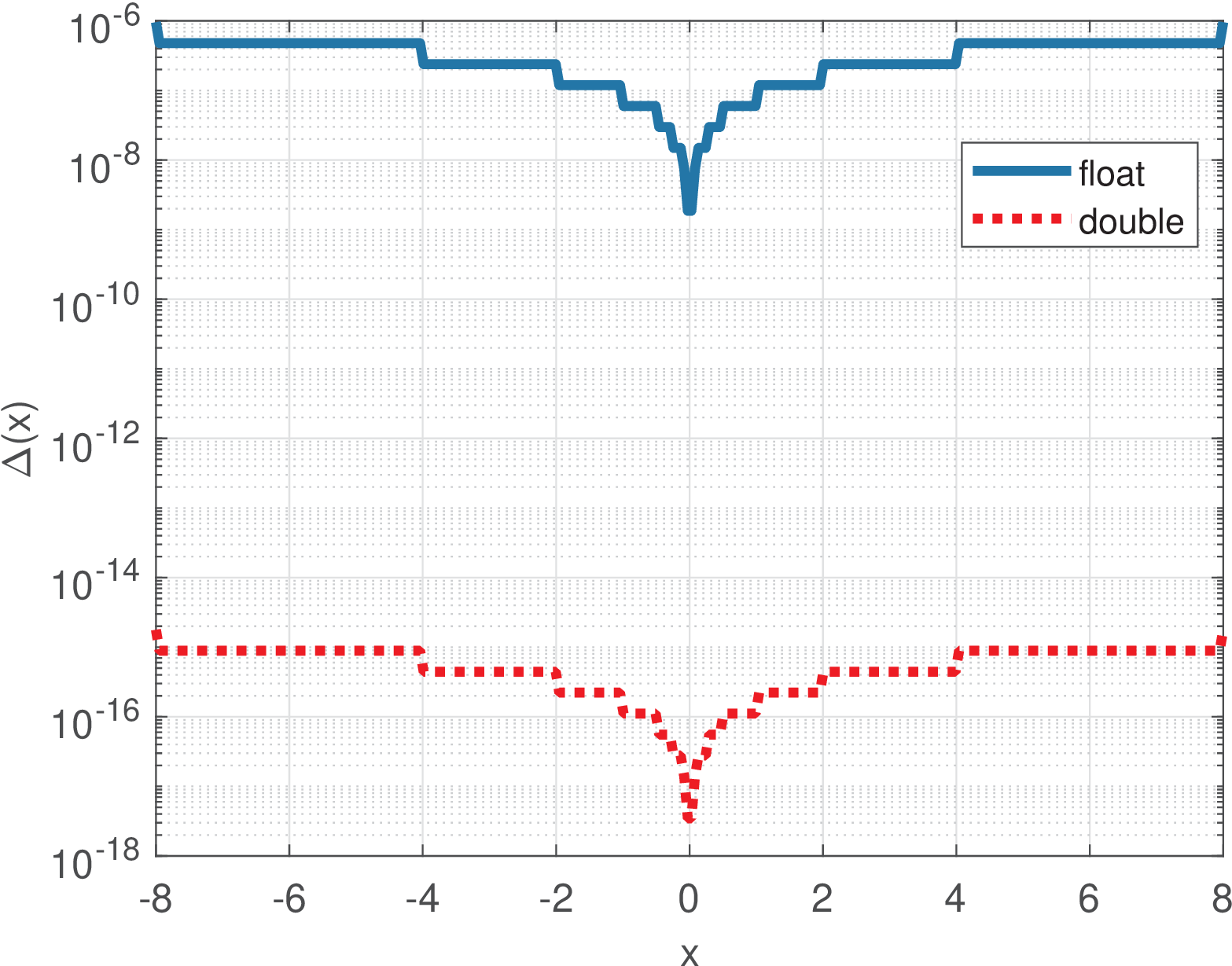
Given that the step $\mathrm{\Delta }(x)$ varies from a number $x$ to the next number $x\; +\mathrm{\Delta }(x)$ in floating point, Matlab/Octave provides the command eps(x) to obtain $\mathrm{\Delta }(x)$. Figure A.36 provides a comparison obtained with Listing A.17.

1N=300; delta_x=zeros(1,N); x=linspace(-8,8,N); %define range 
2%use loops to be compatible with Octave. Matlab allows delta_x=eps(x) 
3for i=1:N, delta_x(i) = eps(single(x(i))); end %single precision 
4semilogy(x,delta_x); hold on 
5for i=1:N, delta_x(i) = eps(x(i)); end  %double precision 
6semilogy(x,delta_x,'r:'); legend('float','double'); grid

Figure A.36 indicates that care must be exercised especially when dealing with single precision, which is a requirement of many DSP chips, for example. Even double precision can cause strange behavior. A good example is provided by Listing A.18, from Mathwork’s documentation [ url1flm].

1a = 0.0; %a uses double precision 
2for i = 1:20 
3  a = a + 0.1; %20 times 0.1 should be equal to 2 
4end 
5a == 2 %checking if a is 2 returns false due to numerical errors

The design of algorithms that are robust to numerical errors, such as matrix inversion, is the focus of many textbooks. Besides trying to adopt robust algorithms, a DSP programmer needs to always be aware of the possibility of numerical errors. Taking the example of the previous code, instead of a check such as if (a==2), it is often better to write

1if abs(a-2) < eps %check if a is 2 (consider numerical errors)

where eps corresponds to eps(1) and is the default when a better guess for the range of interest (eps(2) in the example) is not available.

It is possible to instruct Matlab/Octave to use single (using the function single) or double precision (the default) as illustrated in Listing A.19, which uses the FFT algorithm (to be discussed in Chapter C.14) to compare the options with respect to speed.

1N=2^20; %FFT length (one may try different values) 
2xs=single(randn(1,N)); %generate random signal using single precision 
3xd=randn(1,N); %generate random signal using double precision 
4tic %start time counter 
5Xs=fft(xs); %calculate FFT with single precision 
6disp('Single precision: '), toc %stop time counter 
7tic %start time counter 
8Xd=fft(xd); %calculate FFT with double precision 
9disp('Double precision: '), toc %stop time counter

Note that benchmarking is tricky and using single precision may not be faster than double precision. On a given laptop, Listing A.19 executed on Matlab returned 0.073124 and 0.104728 seconds, which indicates that double precision was approximately 1.43 times slower than single precision. Executing the code on the same machine using Octave led to approximately 0.06 seconds to both double and single precision.