F.11  Time-frequency Analysis using the Spectrogram

F.11.1  Definitions of STFT and spectrogram

The PSD is a powerful tool to analyze signals in the frequency-domain. However, a single PSD fails when the signal “changes” over time. More strictly, if the signal cannot be assumed (WSS) stationary, alternative tools are potentially needed to describe how information varies in frequency and time domains. One relatively simple technique is the short-time Fourier transform (STFT).

The concept behind STFT is to extract segments of the signal under analysis using windowing and calculate several Fourier transforms, one for each segment. Mathematically, the STFT of a continuous-time signal $x(t)$ is

where $\tau$ is used to shift the window $w(t)$ originally centered at $t\; =\; 0$. Eq. (F.68) can be interpreted by fixing $\tau \; ={\tau }_0$ and observing that $X({\tau }_0,f)$ is the Fourier transform of the windowed signal $x(t)w(t\; -{\tau }_0)$. The STFT is invertible and allows for recovering $x(t)$. However, in the sequel it is assumed that the phase can be discarded given that the main interest is to observe the distribution of power along frequency and time.

The spectrogram (for continuous-time)

is defined as the squared magnitude of the STFT and is widely used to analyze nonstationary signals. The specgram function in Matlab/Octave can be used to estimate spectrograms $S(\tau ,\mathrm{\Omega })$ for discrete-time signals. Because $S(\tau ,\mathrm{\Omega })$ is restricted to real numbers, a color scale can be used instead of a 3-d graph. Two examples of spectrograms are provided in Figure C.9 and Figure C.10. The burst of power spread over the whole bandwidth at approximately $n\; =\; 1500$ in Figure C.9 occurs because the windowed signal at this specific FFT is composed by incomplete cycles of both cosines. Note also in Figure C.10, the bursts of power at the transitions between symbols.

F.11.2  Advanced: Wide and narrowband spectrograms

A fundamental restriction of the STFT and, consequently, spectrograms, is the tradeoff between time and frequency resolution. When the window is made longer (its duration is increased), the frequency resolution improves but the time resolution gets worse. A spectrogram is called narrowband when the window is long and the FFT invoked by the spectrogram routine is equivalent to a bank of filters (see Section F.3.2.0) with relatively narrow bandwidth. In contrast, a wideband spectrogram uses a short window and, consequently, the FFT corresponds to filters with relatively large bandwidths. The two spectrograms are contrasted here via an example using a speech signal. Speech is highly non stationary given that the information regarding the phonemes is encoded in segments composed of distinct frequencies. The sentence “We were away” was recorded with $F_s=\; 8000$ Hz using the Audacity free software and stored as a (RIFF) wav file.

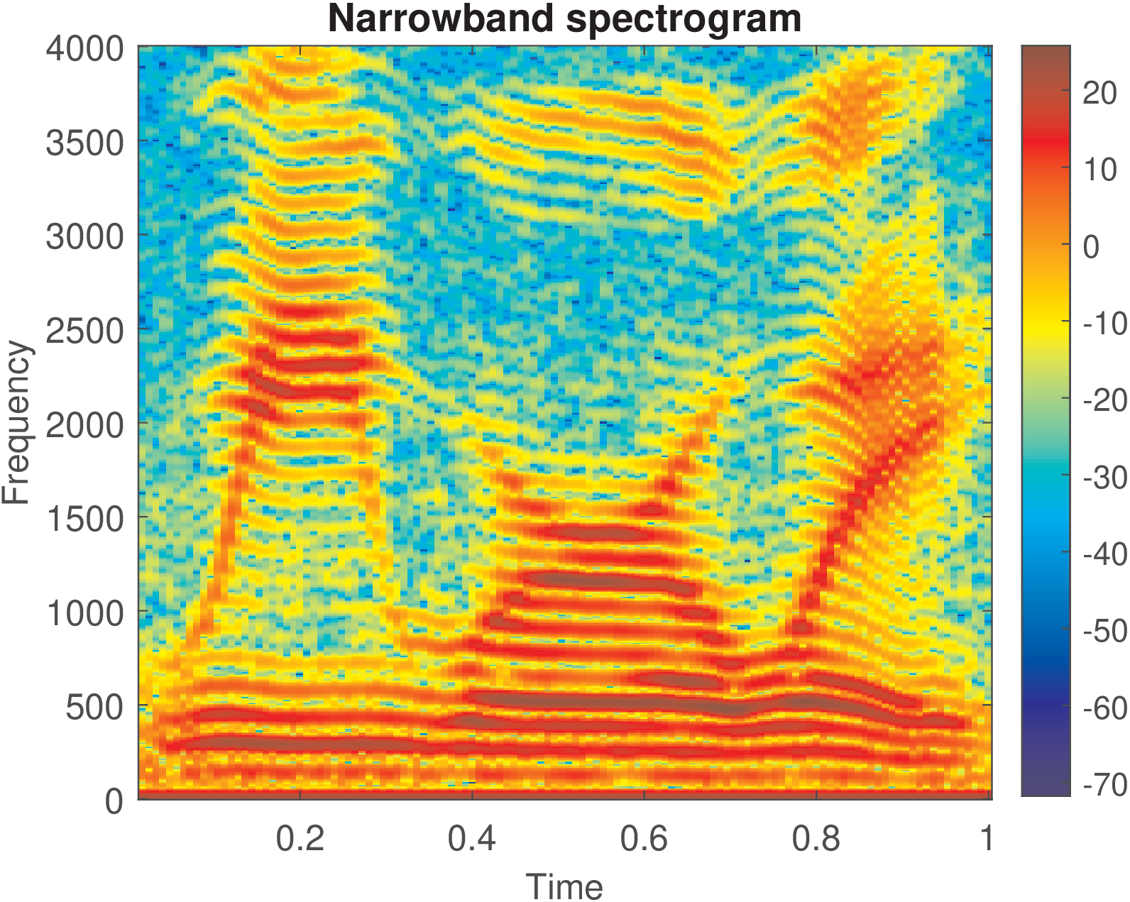
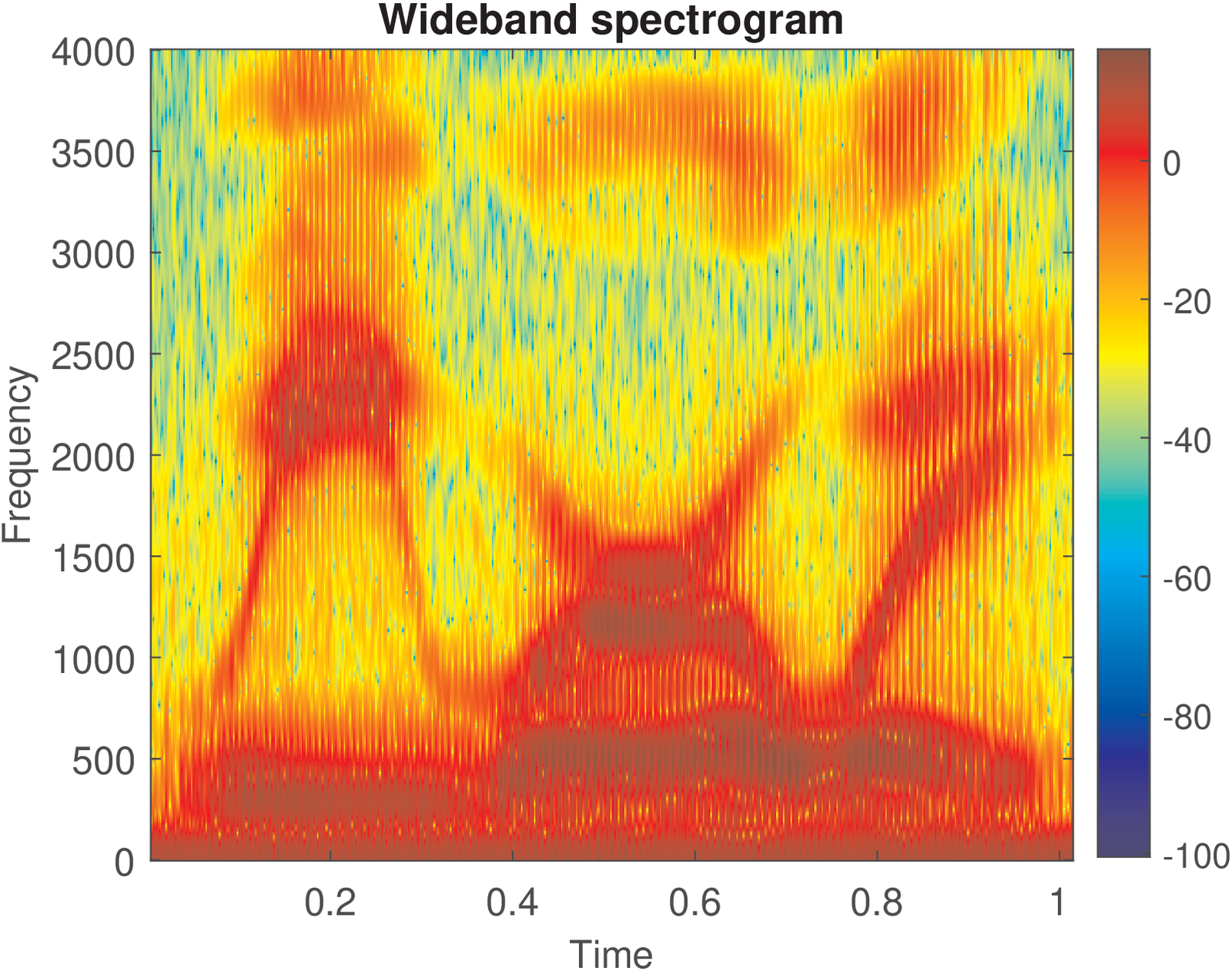
Figure F.41 and Figure F.42 were generated with Listing F.27.

1[s,Fs,wmode,fidx]=readwav('WeWereAway.wav','r'); %read wav file 
2numbits = fidx(7); % num of bits per sample (should be 16) 
3Nfft = 1024; %number of FFT points 
4figure(1), M=64; %window length in samples for wideband 
5specgram(s,Nfft,Fs,hann(M),round(3/4*M)); colorbar 
6figure(2), M=256; %window length in samples for narrowband 
7specgram(s,Nfft,Fs,hann(M),round(3/4*M)); colorbar

Figure F.42 shows a broadband spectrogram (good time resolution but poor frequency resolution) calculated with frames of 64 samples obtained by a Hann window. The frames had an overlap of 3/4 of the frame size, and the spectrum of each windowed signal is calculated through a 1024-point FFT. Zero-padding was used (1024 instead of 64) in order to sample more densely the DTFT of the windowed signal. The user is invited to try the command specgram(s,M,Fs,hann(M),0), which corresponds to not using zero-padding and overlapping to notice the improvements these two strategies bring.

Figure F.41 simply increases the window length from 64 to 256 to create a narrowband spectrogram (poor time resolution and good frequency resolution). The narrowband version allows to see the harmonic structure due to the pitch (see Application C.10) as horizontal strips in the graph. This harmonic structure appears in Figure F.42 as vertical strips.