An Introduction to Quantization

C.9 An Introduction to Quantization

Similar to sampling, quantization is very important, for example, because computers and other digital systems use a limited number $b$ of bits to represent numbers. In order to convert an analog signal to be processed by a computer, it is therefore necessary to quantize its sampled values.

Quantization is used not only when ADCs are involved. Whenever it is necessary to perform an operation representing the numbers with less bits than the current representation, this process can be modeled as quantization. For instance, an image with the pixels represented by 8 bits can be turned into a binary image with a quantizer that outputs one bit. Or an audio signal stored as a WAV file can be converted from 24 to 16 bits per sample.

C.9.1 Quantization definitions

A quantizer $Q$ maps input values from a set (eventually with an infinite number of elements) to a smaller set with a finite number of elements. Without loss of generality, one can assume in this text that the quantizer inputs are real numbers. Hence, the quantizer is described as a mapping $Q : ℝ → ℳ$ from a real number $x[n] ∈ ℝ$ to an element $x_{q} [n]$ of a finite set $ℳ$ called codebook. The quantization process can be represented pictorially by:

x[n]→ Q → x_{q} [n] ∈ ℳ .

The cardinality of this set is $|ℳ | = M$ and typically $M = 2^{b}$ , where $b$ is the number of bits used to represent each output $x_{q} [n]$ . The higher $b$ , the more accurate the representation tends to be.

A generic quantizer can then be defined by the quantization levels specified in $ℳ$ and the corresponding input range that is mapped to each quantization level. These ranges impose a partition of the input space. Most practical quantizers impose a partition that corresponds to rounding the input number to the nearest output level. An alternative to rounding is truncation and, in general, the quantizer mapping is arbitrary.

The input/output relation of most quantizers can be depicted as a “stairs” graph, with a non-linear mapping describing the range of input values that are mapped into a given element of the output set $ℳ$ .

Example C.38. Example of generic (non-uniform) quantizer. For instance, assuming the codebook is $ℳ = {−4,−1,0,3}$ and a quantizer that uses “rounding” to the nearest output level, the input/output mapping is given by Figure C.46.

Figure C.46: Input/output mapping for the non-uniform quantizer specified by $ℳ = {−4,−1,0,3}$ .

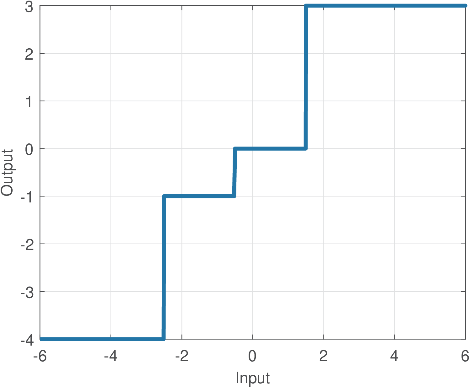
Table C.6 lists the input ranges and corresponding quantizer output levels for the example of Figure C.46.

Table C.6: Input/output mapping for the quantizer specified by

ℳ   = {−4,−1,0,3}

of Figure C.46.


Input range	Output level

$] −∞,−2.5[$	$−4$

$[−2.5,−0.5[$	$−1$

$[−0.5,1.5[$	$0$

$[1.5,∞[$	$3$

Given the adopted rounding, the input thresholds (in this case, $− 2.5$ , $− 0.5$ and $1.5$ ) indicate when the output changes, and are given by the average between two neighboring output levels. For instance, the threshold $− 2.5 = (−1 − (−4))∕2$ is the average between the outputs $− 4$ and $− 1$ . $□$

The adopted convention is that the input intervals are left-closed and right-open (e. g., $[−2.5,−0.5[$ in Table C.6).

In most practical quantizers, the distance between consecutive output levels is the same and the quantizer is called uniform. In contrast, the quantizer of Table C.6 is called non-uniform.

The quantization error is

e_{q} [n] ≜ x[n] − x_{q} [n].

Example C.39. Examples of rounding and truncation. Assume the grades of an exam need to be represented by integer numbers. Using rounding and truncation, an original grade of 8.7 is quantized to 9 and 8, respectively. In this case, the quantization error is $− 0.3$ and $0.7$ , respectively. Assuming the original grade can be any real number $x[n] ∈ [0,10]$ , rounding can generate quantization errors in the range $e_{q} [n] ∈ [−0.5,0.5[$ while truncation generates errors $e_{q} [n] ∈ [0,1]$ . $□$

Unless otherwise stated, hereafter we will assume the quantizer implements rounding.

C.9.2 Implementation of a generic quantizer

A quantizer can be implemented as a list of if/else rules implementing a binary search. The quantizer of Table C.6 can be implemented as in Listing C.15.

Listing C.15: MatlabOctaveCodeSnippets/snip_signals_nonuniform_quantization.m. [ Python version]

1x=-5 %define input 
2if x < -0.5 
3    if x < -2.5 
4        x_quantized = -4 %output if x in ]-Inf, -2.5[ 
5    else 
6        x_quantized = -1 %output if x in [-2.5, -0.5[ 
7    end 
8else 
9    if x < 1.5 
10        x_quantized = 0 %output if x in [-0.5, 1.5[ 
11    else 
12        x_quantized = 3 %output if x in [1.5, Inf[ 
13    end 
14end

An alternative implementation of quantization is by performing a “nearest-neighbor” search: find the output level $x_{q} [n]$ minimum squared error between the input value $x[n]$ and all output levels (that play the role of “neighbors” of the input value). This is illustrated in Listing C.16.

Listing C.16: MatlabOctaveCodeSnippets/snip_signals_nonuniform_quant2.m. [ Python version]

1x=2.3 %define input 
2output_levels = [-4, -1, 0, 3]; 
3squared_errors = (output_levels - x).^2; 
4[min_value, min_index] = min(squared_errors); 
5x_quantized = output_levels(min_index) %quantizer output

C.9.3 Uniform quantization

Unless otherwise stated, this text assumes uniform quantizers with a quantization step or step size $Δ$ .

In this case, all the steps in the quantizer “stairs” have both height and width equal to $Δ$ . In contrast, note that the steps in Figure C.46 are not equal. Uniform quantizers are very useful because they are simpler than the generic non-uniform quantizer.

A uniform quantizer is defined by the number $b$ of bits and only two other numbers: $Δ$ and ${\hat{X}}_{min}$ , where ${\hat{X}}_{min}$ is the minimum value of the quantizer output $x_{q} [n] ∈ ℳ$ , where

ℳ   = {{\hat{X}}_{min}, {\hat{X}}_{min} + Δ, {\hat{X}}_{min} + 2 Δ,…, {\hat{X}}_{min} + (M − 1) Δ}.

(C.41)

For instance, assuming $b = 2$ bits, ${\hat{X}}_{min} = −4$ and $Δ = 3$ , the output levels are $ℳ = {−4,−1,2,5}$ .

The value of $Δ$ is also called the least significant bit (LSB) of the ADC, because it represents the value (e. g., in volts) that corresponds to a variation of a single bit. Later, this is also emphasized in Eq. (C.47) in the context of modeling the representation of real numbers in fixed-point as a quantization process.

C.9.4 Granular and overload regions

There are three regions of operation of a quantizer: the granular and two overload (or saturation) regions. An overload region is reached when the input $x[n]$ falls outside the quantizer output dynamic range. The granular is between the two overload regions.

Figure C.47 depicts the input/output relation of a 3-bits quantizer with $Δ = 1$ . In Figure C.47, because $Δ = 1$ , operation in the granular region corresponds to the rounding operation round to the nearest integer. For example, round(2.4)=2 and round(2.7)=3. When $Δ ≠1$ , the quantization still corresponds to rounding to the nearest $\hat{X} ∈ ℳ$ , but $\hat{X}$ is not restricted to be an integer anymore.

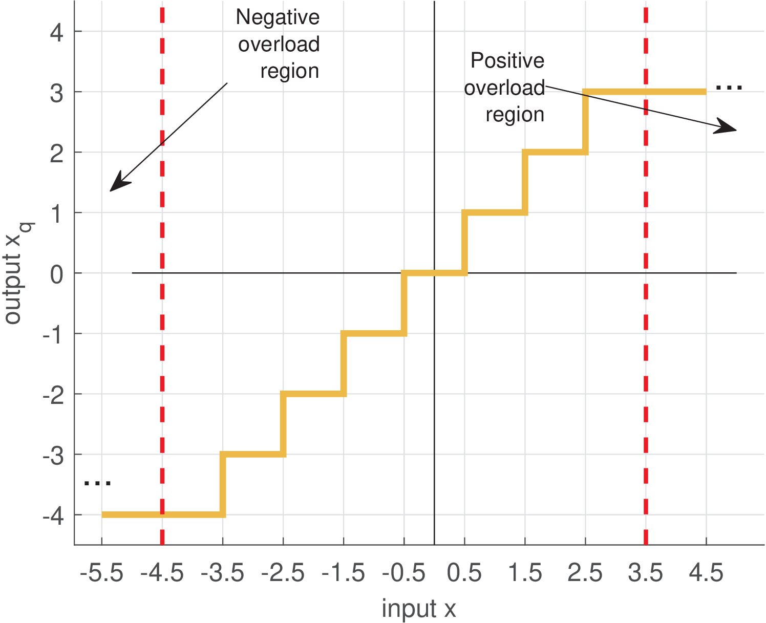
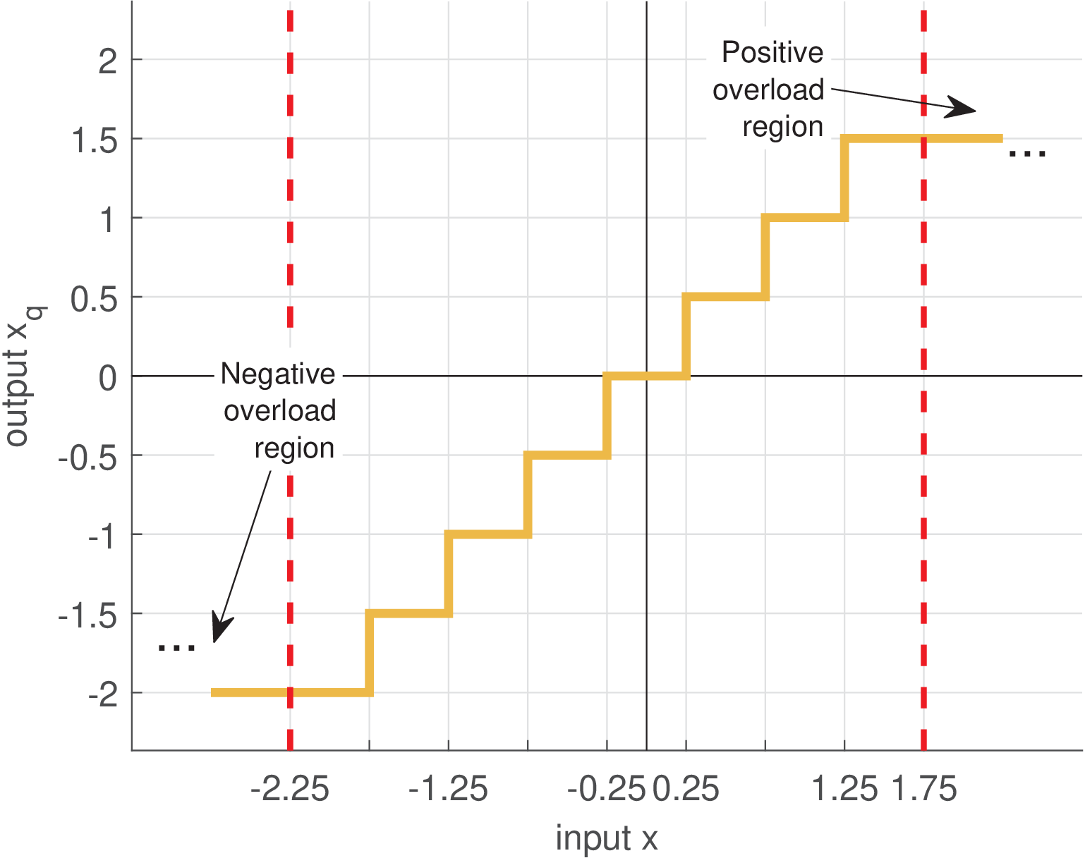
Figure C.47: Input/output relation of a 3-bits quantizer with $Δ = 1$ .

Figure C.48 depicts the input/output relation of a 3-bits quantizer with $Δ = 0.5$ . Close inspection of Figures C.47 and C.48 shows that the error $e_{q} [n]$ is in the range $[− Δ ∕2, Δ ∕2]$ within the granular region, but can grow indefinitely when the input falls in one of the overload regions.

Figure C.48: Input/output relation of a 3-bits quantizer with $Δ = 0.5$ .

C.9.5 Design of uniform quantizers

There are several strategies for designing a uniform quantizer. Some are discussed in the following paragraphs.

Designing a uniform quantizer based on input’s statistics

Ideally, the chosen output levels in $ℳ$ should match the statistics of the input signal $x[n]$ . A reasonable strategy is to observe the histogram (see Figure C.20, for an histogram example) of the quantizer input and pick reasonable values to use in $ℳ$ . For example, if the input data follows a Gaussian distribution, the sample mean $μ$ and variance $σ^{2}$ can be estimated and the dynamic range assumed to be $X_{min} = μ − 3σ$ and $X_{max} = μ + 3σ$ to have the quantizer covering approximately 99% of the samples.

In case the input data has approximately a uniform distribution, the quantizer can be designed based on the dynamic range $[X_{min}, X_{max}]$ of its input $x[n]$ , where $X_{min}$ and $X_{max}$ are the minimum and maximum amplitude values assumed by $x[n]$ .

One should notice that outliers (a sample numerically distant from the rest of the data, typically a noisy sample) can influence too much a design strictly based on $X_{min}$ and $X_{max}$ . This suggests always checking the statistics of $x[n]$ via a histogram.

Designing a uniform quantizer based on input’s dynamic range

Even if the input signal does not have a uniform distribution, it is sometimes convenient to adopt the suboptimal strategy of taking into account only the input dynamic range $[X_{min}, X_{max}]$ of $x[n]$ . Among several possible strategies, a simple one is to choose ${\hat{X}}_{min} = X_{min}$ and

Δ = | \frac{X_{max} − X_{min}}{M} | .

(C.42)

In this case, the minimum quantizer output is ${\hat{X}}_{min} = X_{min}$ , but the maximum value does not reach $X_{max}$ and is given by ${\hat{X}}_{max} = X_{max} − Δ$ . The reason is that, as indicated in Eq. (C.41), ${\hat{X}}_{max} = {\hat{X}}_{min} + (M − 1) Δ$ .

To design a uniform quantizer in which ${\hat{X}}_{max} = X_{max}$ , one can adopt

Δ = | \frac{X_{max} − X_{min}}{M − 1} | .

(C.43)

Example C.40. Design of a uniform quantizer. For example, assume the quantizer should have $b = 2$ bits and the input $x[n]$ has a dynamic range given by $X_{min} = −1$ V and $X_{max} = 3$ V. Using Eq. (C.42) leads to $Δ = (3 − (−1))∕4 = 1$ V and the quantizer output levels are $ℳ = {−1,0,1,2}$ . Note that ${\hat{X}}_{max} = X_{max} − Δ = 3 − 1 = 2$ . Alternatively, Eq. (C.43) can be used to obtain $Δ = (3 − (−1))∕(4 − 1) ≈ 1.33$ V and the quantizer output levels would be $ℳ = {−1,0.33,1.66,3}$ with ${\hat{X}}_{max} = X_{max} = 3$ . $□$

Example C.41. Forcing the quantizer to have an output level representing “zero”. One common requirement when designing a quantizer is to reserve one quantization level to represent zero (otherwise, it would output a non-zero value even with no input signal). The levels provided by Eq. (C.43) can be refined by counting the number $M_{neg}$ of levels representing negative numbers and adjusting ${\hat{X}}_{min}$ such that ${\hat{X}}_{min} + Δ M_{neg} = 0$ . Listing C.17 illustrates the procedure.

Listing C.17: MatlabOctaveCodeSnippets/snip_signals_quantizer.m. [ Python version]

1Xmin=-1; Xmax=3; %adopted minimum and maximum values 
2b=2; %number of bits of the quantizer 
3M=2^b; %number of quantization levels 
4delta=abs((Xmax-Xmin)/(M-1)); %quantization step 
5QuantizerLevels=Xmin + (0:M-1)*delta %output values 
6isZeroRepresented = find(QuantizerLevels==0); %is 0 there? 
7if isempty(isZeroRepresented) %zero is not represented yet 
8    Mneg=sum(QuantizerLevels<0); %number of negative 
9    Xmin = -Mneg*delta; %update the minimum value 
10    NewQuantizerLevels = Xmin + (0:M-1)*delta %new values 
11end

Considering again Example C.40, Listing C.17 would convert the original set $ℳ = {−1,0.33,1.66,3}$ into $ℳ = {−1.33,0,1.33,2.67}$ , which has one level dedicated to represent zero. $□$

Example C.42. Designing a quantizer for a bipolar input.

Assume here a bipolar signal $x[n]$ , for instance with peak values $X_{min} = −5$ and $X_{max} = 5$ ). If it can be assumed that $X_{max} = | X_{min} |$ , Eq. (C.43) simplifies to

Δ = \frac{2 X_{max}}{M − 1} .

Furthermore, one quantization level can be reserved to represent zero, while $M∕2 = 2^{b−1}$ and $M∕2 − 1 = 2^{b−1} − 1$ levels represent negative and positive values, respectively. Most ADCs adopt this division of quantization levels when operating with bipolar inputs. For example, several commercial 8-bits ADCs can output signed integers from $− 128$ to 127, which corresponds to the integer range $− 2^{b−1} = − 2^{8−1} = −128$ to $2^{b−1} − 1 = 2^{7} − 1 = 127$ . These integer values can be multiplied by the quantization step $Δ$ in volts to convert the quantizer output into a value in volts.

Listing C.18 illustrates a Matlab/Octave function that implements a conventional quantizer with ${\hat{X}}_{min} = − 2^{b−1} Δ$ and saturation. The round function is invoked to obtain the integer that represents the number of quantization levels as

x_{i} = round (\frac{x}{Δ}),

(C.44)

and later $x_{q} = x_{i} × Δ$ .

Listing C.18: MatlabOctaveFunctions/ak_quantizer.m

1function [x_q,x_i]=ak_quantizer(x,delta,b) 
2% function [x_q,x_i]=ak_quantizer(x,delta,b) 
3%This function assumes the quantizer allocates 2^(b-1) levels to 
4%negative output values, one level to the "zero" and 2^(b-1)-1 to 
5%positive values. See ak_quantizer2.m for more flexible allocation. 
6%The output x_i will have negative and positive numbers, which 
7%correspond to encoding the quantizer's output with two's complement. 
8x_i = x / delta; %quantizer levels 
9x_i = round(x_i); %nearest integer 
10x_i(x_i > 2^(b-1) - 1) = 2^(b-1) - 1; %impose maximum 
11x_i(x_i < -2^(b-1)) = -2^(b-1); %impose minimum 
12x_q = x_i * delta;  %quantized and decoded output

Listing C.19: MatlabOctaveCodeSnippets/snip_signals_quantizer_use.m. [ Python version]

1delta=0.5; %quantization step 
2b=3; %number of bits, to be used here as range -2^(b-1) to 2^(b-1)-1 
3x=[-5:.01:4]; %define input dynamic range 
4[xq,x_integers] = ak_quantizer(x,delta,b); %quantize 
5plot(x,xq), grid    %generate graph

The commands in Listing C.19 can generate a quantizer input-output graph such as Figure C.48 using the function ak_quantizer.m. $□$

C.9.6 Design of optimum non-uniform quantizers

The optimum quantizer, which minimizes the quantization error, must be designed strictly according to the input signal statistics (more specifically, the probability density function of $x[n]$ ). The uniform quantizer is the optimum only when the input distribution is uniform. For any other distribution, the Lloyd’s algorithm¹⁵ can be used to find the optimum set $ℳ$ of output levels and the quantizer will be non-uniform. For instance, if the input is Gaussian, the optimum quantizer allocates a larger number of quantization levels around the Gaussian mean than in regions far from the mean.

Example C.43. Optimum quantizer for a Gaussian input. This example illustrates the design of an optimum quantizer when the input $x[n]$ has a Gaussian distribution with variance $σ^{2} = 10$ . It is assumed that the number $b$ of bits is three such that the quantizer has $M = 2^{3} = 8$ output levels. The following code illustrates the generation of $x[n]$ and quantizer designer using Lloyd’s algorithm.

1clf 
2N=1000000; %number of random samples 
3b=3; %number of bits 
4variance = 10; 
5x=sqrt(variance)*randn(1,N); %Gaussian samples 
6M=2^b; 
7[partition,codebook] = lloyds(x,M); %design the quantizer

The obtained results are listed in Table C.7 and Figure C.49.

Table C.7: Input/output mapping for a generic quantizer designed for a Gaussian input with variance

σ^{2} = 10


Input range	Output level

$] −∞,−5.5[$	$−6.8$

$[−5.5,−3.3[$	$−4.2$

$[−3.3,−1.6[$	$−2.4$

$[−1.6,0[$	$−0.8$

$[0,1.6[$	$0.8$

$[1.6,3.3[$	$2.4$

$[3.3,5.5[$	$4.2$

$[5.5,∞[$	$6.8$

Note that the two intervals close to 0 have length 1.6 while the interval $[3.3,5.5[$ has a longer length $5.5 − 3.3 = 2.2$ . In general, the intervals corresponding to regions with less probability are longer such that more output levels can be concentrated in regions of high probability. This is illustrated in Figure C.49.

Figure C.49: Theoretical and estimated Gaussian probability density functions with thresholds represented by dashed lines and the output levels indicated with circles in the abscissa.

Because Lloyd’s algorithm has a set of samples as input, this number has to be large enough such that the input distribution is properly represented. In this example, N=1000000 random samples were used.

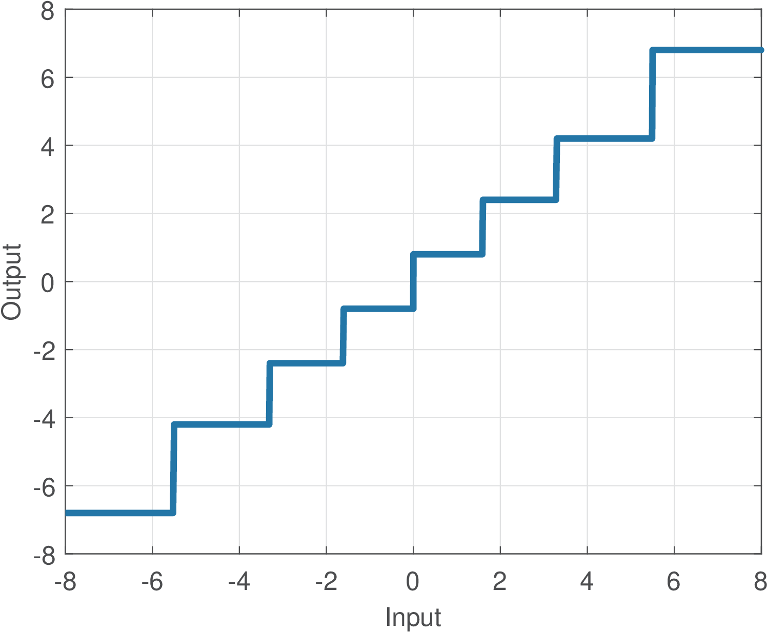
Figure C.50: Input/output mapping for the quantizer designed with a Gaussian input and outputs given by $ℳ = [−6.8,−4.2,−2.4,−0.8,0.8,2.4,4.2,6.8]$ .

Figure C.49 depicts the mapping for the designed non-uniform quantizer. $□$

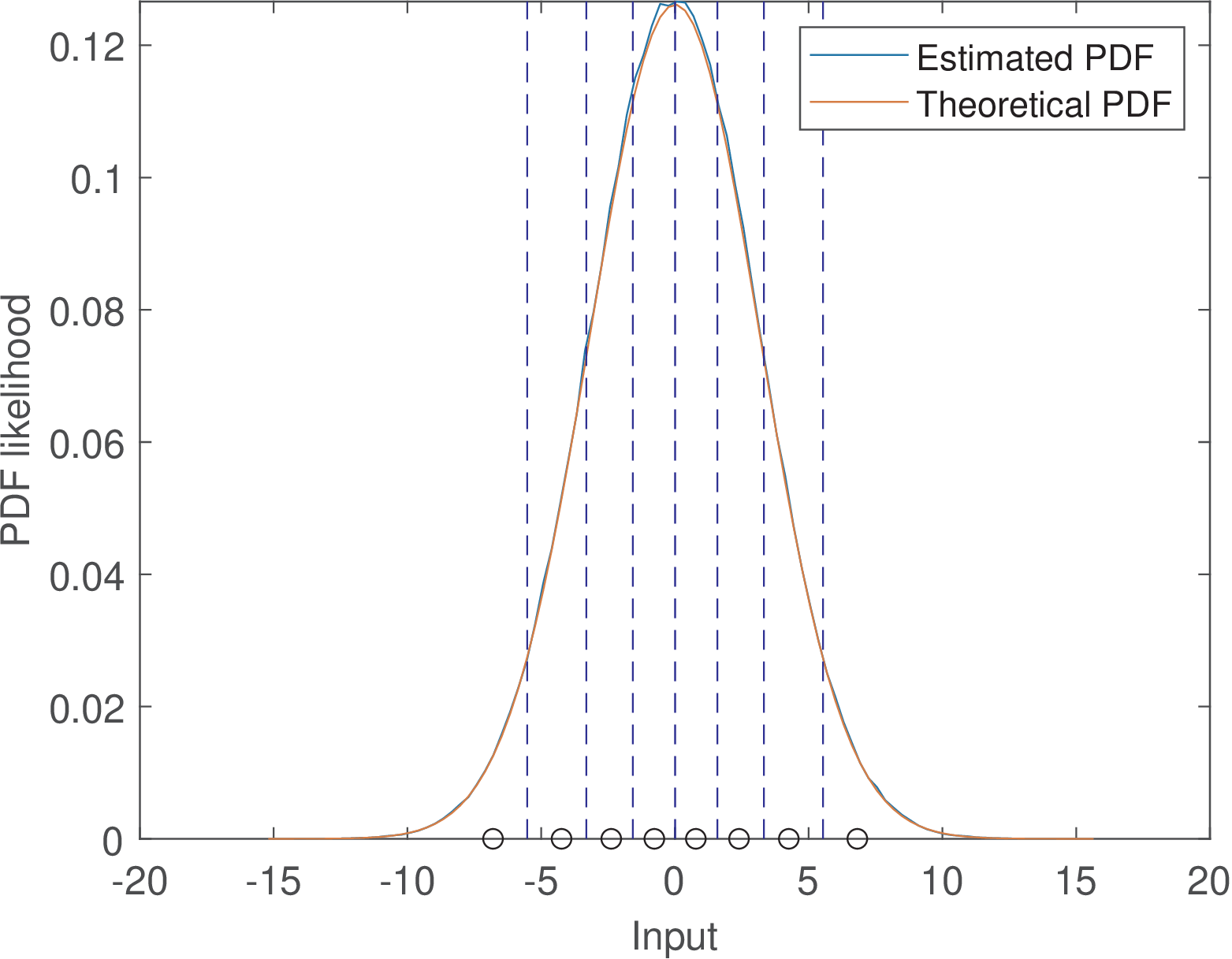
Example C.44. Optimum quantizer for a mixture of two Gaussians. This example is similar to Example C.43, but the input distribution here is a mixture of two Gaussians instead of a single Gaussian. More specifically, the input $x[n]$ has a probability density function given by

f(x) = 0.8 N(−4,0.5) + 0.2 N(3,4),

(C.45)

where the notation $N(μ, σ^{2})$ describes a Gaussian with average $μ$ and variance $σ^{2}$ .

Figure C.51: Results for the quantizer designed with the mixture of Eq. (C.45) as input.

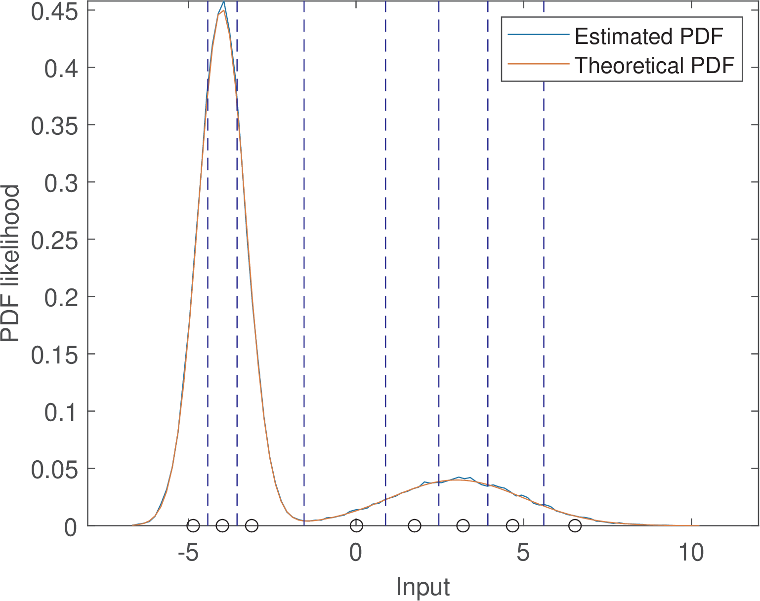
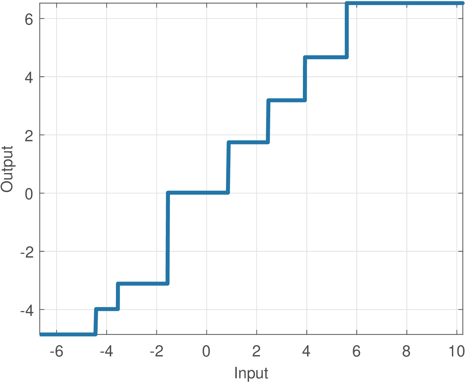
Figure C.51 illustrates results obtained with the Lloyd’s algorithm (see script figs_signals_quantizer.m). Figure C.51 indicates that three quantizer levels are located closer to the Gaussian with average $μ = −4$ , while the other five levels are dedicated to the Gaussian with $μ = 3$ . Because the input distribution is the mixture of Gaussians of Eq. (C.45), quantization steps are smaller around the input $x = −4$ , and larger around $x = 3$ . The largest step height occurs in a region close to $x = −1$ due to the relatively low probability in this region. $□$

C.9.7 Quantization stages: classification and decoding

Recall that the complete A/D process to obtain a digital signal $x_{q} [n]$ to represent an analog signal $x(t)$ can be modeled as:

x(t)→ SAMPLING → x_{s} (t)→ S∕D →x[n]→ Q → x_{q} [n].

Note the convention adopted for the quantizer output: $x_{q} [n]$ is represented by real numbers, as in Listing C.18. This is convenient because one wants to perform signal processing with $x_{q} [n]$ , for instance, calculating the quantization error with $e_{q} [n] = x[n] − x_{q} [n]$ . However, in digital hardware, a binary representation $x_{b} [n]$ better describes the actual output of an ADC. Hence, a more faithful representation of the job actually done by the ADC should be denoted as

x(t)→ SAMPLING → x_{s} (t)→ S∕D →x[n] → {\tilde{Q}}_{c} → x_{b} [n],

where ${\tilde{Q}}_{c}$ generates binary codewords, not real numbers. Hence, to enable better representing an ADC output and related variables, the quantization is broken into the two stages depicted in Figure C.52: classification and decoding, denoted as ${\tilde{Q}}_{c}$ and ${\tilde{Q}}_{d}$ , respectively.

Figure C.52: A quantizer $Q$ is composed by the classification and decoding stages, denoted as ${\tilde{Q}}_{c}$ and ${\tilde{Q}}_{d}$ , respectively.

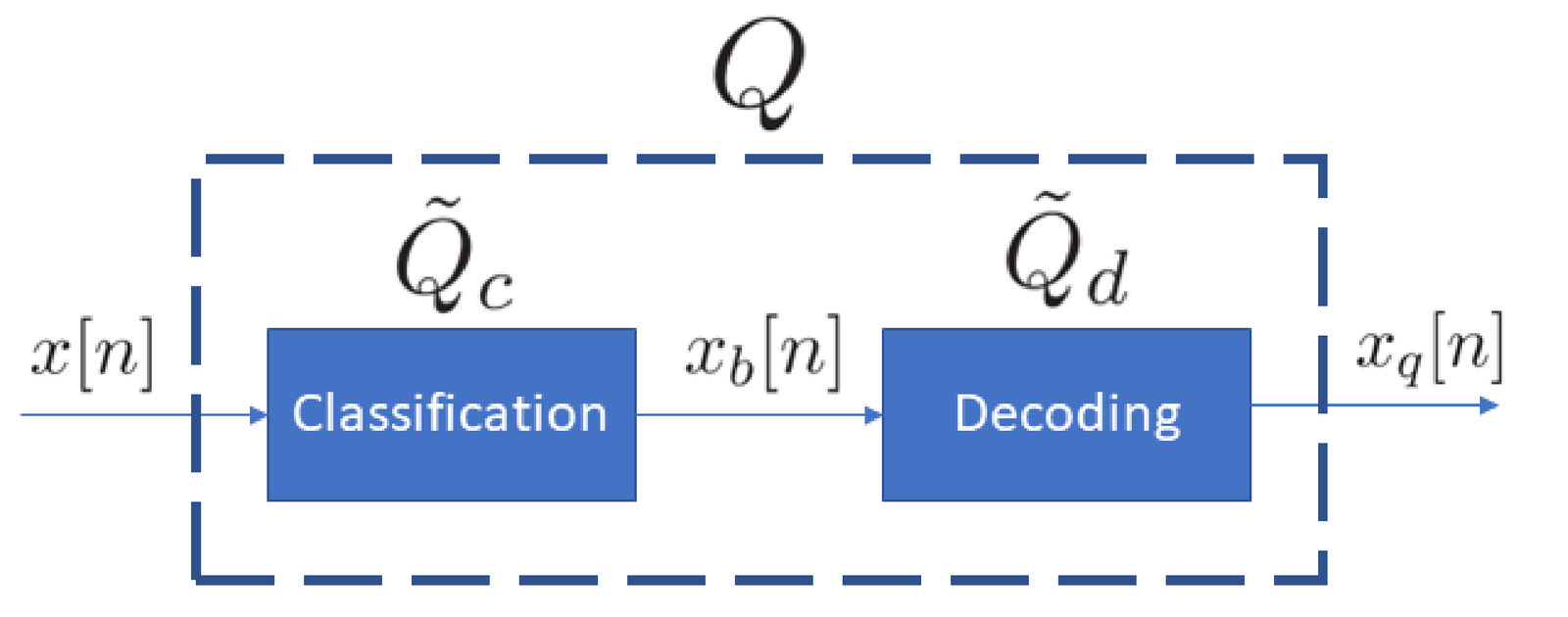
The output ${\tilde{Q}}_{c} {x[n]}$ of the classification stage is represented by a binary codeword $x_{b} [n]$ with $b$ bits. The decoding corresponds to obtaining a real number using $x_{q} [n] = {\tilde{Q}}_{d} {x_{b} [n]}$ . The next section discusses the decoding stage.

C.9.8 Binary numbering schemes for quantization decoding

The decoding mapping ${\tilde{Q}}_{d} {⋅}$ in Figure C.52 can be arbitrary, but in most cases simple and well-known binary numbering schemes are adopted. When assuming a quantizer that uses bipolar inputs (see Eq. (C.44)), decoding often relies on a binary numbering scheme that is able of representing negative numbers. Otherwise, an unsigned numbering scheme is adopted. In both cases, the numbering scheme allows to convert $x_{b} [n]$ into an integer $x_{i} [n]$ , represented in the decimal system.

As the final decoding step, the integer $x_{i} [n]$ is multiplied by the quantization step $Δ$ , as indicated in Example C.42 and repeated below:

x_{q} [n] = {\tilde{Q}}_{d} {x_{b} [n]} = x_{i} [n] × Δ .

(C.46)

There are various binary numeral systems that differ specially on how negative numbers are represented. Some options are briefly discussed in the sequel.¹⁶ Table C.8 provides an example of practical binary numbering schemes, also called codes. The first column indicates values for $x_{b}$ while the others indicate $x_{i}$ values. For example, note in Table C.8 that $x_{b} [n] = 100$ corresponds to 7 in Gray code and $− 4$ in two’s complement.

Table C.8: Examples of binary numbering schemes used as output codes in A/D conversion for

b = 3

bits.

Binary number	Unsigned integer	Two’s complement	Offset	Sign and magnitude	Gray code
$000$	$0$	$0$	$−4$	$0$	$0$
$001$	$1$	$1$	$−3$	$1$	$1$
$010$	$2$	$2$	$−2$	$2$	$3$
$011$	$3$	$3$	$−1$	$3$	$2$
$100$	$4$	$−4$	$0$	$“ −0 ”$	$7$
$101$	$5$	$−3$	$1$	$−1$	$6$
$110$	$6$	$−2$	$2$	$−2$	$4$
$111$	$7$	$−1$	$3$	$−3$	$5$

Three of the codes exemplified in Table C.8 will be discussed in more details because they are very important from a practical point of view: unsigned integer, offset and two’s complement output coding.

The unsigned representation, sometimes called standard-positive binary coding, represents numbers in the range $[0, 2^{b} − 1]$ . It is simple and convenient for arithmetic operations such as addition and subtraction. However, it cannot represent negative values. An alternative is the offset representation, which is capable of representing numbers in the range $[− 2^{b−1}, 2^{b−1} − 1]$ , as used in Listing C.18. This binary numbering scheme can be obtained by subtracting the “offset” $2^{b−1}$ from the unsigned representation. The two’s complement is a popular alternative that is also capable of representing numbers in the range $[− 2^{b−1}, 2^{b−1} − 1]$ and allows for easier arithmetics than the offset representation, as studied in textbooks of digital electronics. Note that the offset representation can be obtained by inverting the most significant bit (MSB) of the two’s complement. For this reason it is sometimes called offset two’s complement.

Example C.45. Negative numbers in two’s complement. To represent a negative number in two’s complement, one can first represent the absolute value in standard-positive binary coding, then invert all bits and sum 1 to the result. For example, assuming $x_{i} [n] = −81$ should be represented with $b = 8$ bits, the first step would lead to $01010001$ , which corresponds to $81$ . Inverting these bits leads to $10101110$ and summing to 1 gives the final result $x_{b} [n] = 10101111$ corresponding to $− 81$ .

Note that two’s complement requires sign extension (see, e. g., [ url1two]) by extending the MSB. For example, if $x_{i} [n] = −81$ were to be represented with $b = 16$ bits, the first step would lead to $00000000$ $01010001$ , corresponding to $81$ . After inverting the bits to obtain $11111111$ $10101110$ and summing 1, the correct codeword to represent $− 81$ would be $x_{b} [n] = 11111111$ $10101111$ (instead of $00000000$ $10101111$ ). Comparing the representation of $− 81$ in 16 and 8 bits, one can see that the MSB of the 8-bits representation was extended (repeated) in the first byte of the 16-bits version. $□$

Distinguishing $x_{i} [n]$ and $x_{b} [n]$ may seem an abuse of notation because they are the same number described in decimal and binary numeral systems, respectively. However, the notation is useful because there are many distinct ways of mapping $x_{b} [n]$ to $x_{i} [n]$ and vice-versa.

Table C.8 covers the binary numbering schemes adopted in most ADCs. These schemes can be organized within a class of number representation called fixed-point. But the representation of real numbers within computers typically use a more flexible representation belonging to another class called floating-point. The fixed and floating-point representations are discussed in the next subsection.

C.9.9 Representing numbers in fixed-point

Both fixed and floating-point representations are capable of representing real numbers. A real number can be written as the sum of an integer part and a fractional part that is less than one and non-negative.

The name “fixed-point” is due to the fact that the $b$ bits available to represent a number are organized as follows:

1 bit representing the sign (positive or negative) of the integer part and, consequently, of the number itself
$b_{i}$ bits representing the integer part of the number
$b_{f}$ bits representing the fractional part of the number

such that $b = b_{i} + b_{f} + 1$ bits. For simplicity, the sign bit is assumed here to be the MSB, but in practice that depends on the adopted standard and the machine endianness (see [ url1ofi]) for a brief explanation of big and little endian formats).

One way of thinking the “point” is that there is flexibility on choosing the power of 2 that is associated to the second bit, at the right of the MSB. After this design choice is made, a fictitious point separates the bits corresponding to the integer part from the fractional part bits. There is a convention of denoting the values chosen for $b_{i}$ and $b_{f}$ as Q $b_{i}$ . $b_{f}$ .

Figure C.53: Fixed-point representation Q3.4 of the real number 5.0625. The “point” is always after the bit corresponding to the weight $2^{0}$ .

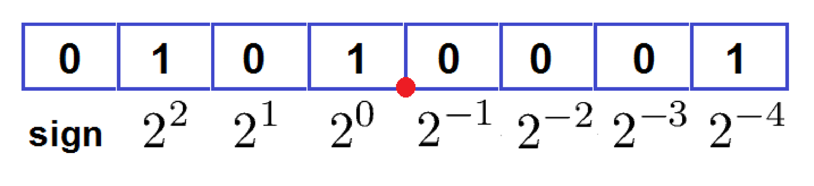
Figure C.53 shows an example of fixed-point representation using Q3.4, for which $b_{i} = 3$ , $b_{f} = 4$ and, consequently $b = 8$ . In this case, the point is located between the fourth and fifth bits. The binary codeword $x_{b} = 01010001$ is mapped to a real number according to the position of the point:

1 × 2^{2} + 0 × 2^{1} + 1 × 2^{0} + 0 × 2^{−1} + 0 × 2^{−2} + 0 × 2^{−3} + 1 × 2^{−4} = 5.0625.

It is very common to normalize the numbers to make them fit the range $[−1,1[$ . In this case $b_{i}$ can be zero, $b_{f} = b − 1$ and the second bit has a weight in base-2 equals to $2^{−1}$ such that the point is between the MSB and this bit. The other bit weights are then $2^{−2},…, 2^{− b_{f}}$ , according to their respective position. For example, the outputs of a quantizer with $b = 2$ bits when represented in the format Q0.1 ( $b_{i} = 0$ , $b_{f} = 1$ ) assume four possible outputs $x_{q} ∈{−1,−0.5,0,0.5}$ . In general, the weight $2^{− b_{f}}$ of the LSB corresponds to the value of the step size, i. e.

Δ = 2^{− b_{f}} .

(C.47)

Note that the number 5.0625 in Figure C.53 can also be obtained by identifying that $x_{b}$ corresponds to $x_{i} = 81$ and calculating $x_{q} = x_{i} Δ = 81 × 2^{−4} = 5.0625$ . If the point were moved to the position between the MSB and second bit, which corresponds to choosing Q0.7, the quantizer would have $Δ = 2^{−7}$ and the same codeword $x_{b} = 01010001$ would be mapped to $x_{q} = 0.6328125$ .

In summary, when a fixed-point representation is assumed, the quantizer has step $Δ = 2^{− b_{f}}$ and can output numbers in the range $[− 2^{b_{i}}, 2^{b_{i}} − Δ]$ . Algorithm 1 describes the process for representing a real number $x$ in fixed-point using Q $b_{i}$ . $b_{f}$ .

______________________________________________________________________________ Algorithm 1: Fixed-point conversion._________________________________________________________ Input:

x

b_{i}

b_{f}

// value to quantize, integer and fractional # bits Output:

x_{b}

x_{i}

x_{q}

// binary, integer and decoded forms of

Q{x}

x_{i} = x∕ Δ

// Equivalent to multiplying by

1∕ Δ = 2^{b_{f}}

2if

x_{i}

is not an integer then 3 4 5round

x_{i}

to the nearest integer // floor is sometimes used instead 6if

x_{i} < − 2^{b_{i}}

then 7 8 9

x_{i} = − 2^{b_{i}}

// Implement saturation for negative values 10Print: Warning! Consider increasing number

b_{i}

of integer bits 11if

x_{i} > 2^{b_{i}} − Δ

then 12 13 14

x_{i} = 2^{b_{i}} − Δ

// Implement saturation for positive values 15Print: Warning! Consider increasing number

b_{i}

of integer bits 16

x_{q} = x_{i} × Δ

// Multiply by

Δ

to find decoded value 17if

x_{i} < 0

then 18 19 20Obtain

x_{b}

using two’s complement // with

b

bits and sign extension 21else 22 23 24Simply obtain

x_{b}

as the standard-positive binary coding of

x_{i}

___

For example, using Algorithm 1 to represent $x = −7.45$ in Q3.4, the first step is to calculate $x∕ Δ = −7.45 × 2^{4} = −119.2$ . Then, using round leads to $x_{i} = −119$ , which corresponds to $x_{q} = −7.4375$ and $x_{b} = 10001001$ in two’s complement. This algorithm is the same implemented in Listing C.18 but explicitly outputs the binary codeword $x_{b}$ .

Choosing the point position depends on the dynamic range of the numbers that will be represented and processed. This is typically done with the help of simulations and is a challenging task due to the tradeoff between range (the larger $b_{i}$ the better) and precision (the larger $b_{f}$ the better). In sophisticated algorithms, it is typically required to assume distinct positions for the point at different stages of the process. In such cases, using specialized tools such as Mathwork’s Fixed-Point Designer [ url1mfi] can significantly help.

Example C.46. Fixed-point in Matlab. Matlab counts with the well-documented Fixed-Point Toolbox. If you have this Matlab’s toolbox, try for example doc fi. The Matlab command for representing $x = −7.45$ as in the previous example is:

1x=-7.45;signed=1;b=8;bf=4;x_q=fi(x,signed,b,bf)

which outputs:

     x_q = -7.437500000000000
               DataTypeMode: Fixed-point: binary point scaling
                     Signed: true
                 WordLength: 8
             FractionLength: 4
                  RoundMode: nearest
               OverflowMode: saturate
                ProductMode: FullPrecision
       MaxProductWordLength: 128
                    SumMode: FullPrecision
           MaxSumWordLength: 128
              CastBeforeSum: true

$□$

Example C.47. Quantization example in Matlab. As another example, let $x(t_{0}) = 2804.6542$ volts be the amplitude of $x(t)$ at $t = t_{0}$ , such that $x[n_{0}] = 2804.6542$ , where $n_{0}$ is the value of $n$ corresponding to $t = n_{0} T_{s}$ . The value of $x[n_{0}]$ quantized with $b = 16$ bits and reserving $b_{i} = 12$ bits to the integer part is $x_{q} [n_{0}] = Q{x[n_{0}]} = 2804.625$ , which can be obtained in Matlab with:

1format long %to better visualize numbers 
2x=2804.6542; %define x 
3xq=fi(x) %quantize with 16 bits and "best-precision" fraction length

When fi is used with a single argument, it assumes a 16-bit word length and it adjusts $b_{f}$ such that the integer part of the number can be represented (called in Matlab “best-precision” fraction length). For this example, the result is:

           xq = 2.804625000000000e+03
           Signedness: Signed
           WordLength: 16
           FractionLength: 3

indicating that $b_{i} = 12$ bits are used to represent the integer part of $x$ (2084), given that $2^{11} = 2048 < x < 2^{12} = 4096$ . Considering one bit is reserved for the sign, then $b_{f} = 16 − 1 − b_{i} = 3$ bits, which is the FractionLength. $□$

C.9.10 IEEE 754 floating-point standard

Choosing the point position provides a degree of freedom for trading off range and precision in a fixed-point representation. However, there are situations in which a software needs to deal simultaneously with small and large numbers, and having distinct positions for the point all over the software is not practical or efficient. For example, if distances in both nanometers and kilometers should be manipulated with reasonable precision, the dynamic range of $1 0^{3} ∕1 0^{−9} = 1 0^{12}$ would require $b_{i} > 40$ bits for the integer part or keeping track of two distinct point positions. Hence, in many cases, a floating-point representation is more adequate.

A number in floating point is represented as in scientific notation:

x_{q} = significand × {base}^{exponent} .

(C.48)

For example, assuming the base is 10 for simplicity, the number $x_{q} = 123.4567$ is interpreted as $x_{q} = 1.234567 × 1 0^{2}$ , where 1.234567 is the significand and 2 the exponent. While in fixed-point the $b − 1$ bits available to represent a signed number are split between $b_{i}$ and $b_{f}$ , in floating point the $b$ bits are split between the significand and exponent.

The key aspect of Eq. (C.48) is that, as the value of the exponent changes, the “point” has new positions and allows to play a different trade off between range and precision: the values a floating point $x_{q}$ can assume are not uniformly spaced. While fixed-point numbers are uniformly spaced by $Δ = 2^{− b_{f}}$ , which then imposes the maximum error within the range, the error magnitude in a floating point representation depends on the value of the exponent. For a given error in the significand representation, the larger the exponent, the larger the absolute error of $x_{q}$ with respect to the number it represents. This is a desired feature in many applications and floating point is used for example in all personal computers. The fixed-point niche are embedded systems, where power consumption and cost have more stringent requirements.

The IEEE 754 standard for representing numbers and performing arithmetics in floating point is adopted in almost all computing platforms. Among other features,¹⁷ it provides support to single and double precision, which are typically called “float” and “double”, respectively, in programming languages such as C and Java.

The wide adoption of IEEE 754 is convenient because a binary file written with a given language in a given platform can be easily read with a distinct language in another platform. In this case, the only concern is to make sure the endianness is the same ([ url1ofi]). Two examples discussing numerical errors and quantization in practical scenarios are presented in Appendix A.31.

C.9.11 Quantization examples

Some quantization examples are provided in the following paragraphs.

Example C.48. ECG quantization. An ECG signal was obtained with a digital Holter that used a uniform quantizer with 8 bits represented in two’s complement and quantization step $Δ = 0.15$ mV. Hence, when represented as decimal numbers, the quantized outputs $x_{i} [n]$ vary from $− 128$ to 127. Assuming three quantizer input samples as $x[0] = 2.52$ , $x[1] = −14.8$ and $x[2] = 7.3$ , all in mV, the quantized values are given by $x_{i} [n] = Q{x[n]} = round (x[n]∕ Δ)$ , which lead to $x_{i} [0] = 17$ , $x_{i} [1] = −99$ and $x_{i} [2] = 49$ . The corresponding binary codewords $x_{b} [n] = {\tilde{Q}}_{c} {x[n]}$ are $x_{b} [0] = 0001 0001$ , $x_{b} [1] = 1001 1101$ and $x_{b} [2] = 0011 0001$ . Using Eq. (C.46), the quantizer outputs are $x_{q} [0] = 2.55$ , $x_{q} [1] = −14.85$ and $x_{q} [2] = 7.35$ mV, and the quantization error $x[n] − x_{q} [n]$ is $e_{q} [0] = −0.03$ , $e_{q} [1] = 0.05$ and $e_{q} [2] = −0.05$ mV. $□$

Example C.49. Quantization using 16 bits. Assume the quantizer of an ADC with $Δ = 0.5$ and $b = 16$ bits is used to quantize the discrete-time signal $x[n]$ at time $n_{0}$ . The input amplitude is $x[n_{0}] = 12804.5241$ and the quantizer output is $Q{x[n_{0}]} = 12804.5$ . It is also assumed that the classification quantizer stage ${\tilde{Q}}_{c}$ outputs $x_{b} [n_{0}] = {\tilde{Q}}_{c} {x[n_{0}]} = 0110 0100 0000 1001$ in two’s complement, which in decimal is $x_{i} [n_{0}] = 25609$ . The decoding then generates

x_{q} [n_{0}] = x_{i} [n_{0}] × Δ = 25609 × 0.5 = 12804.5,

using Eq. (C.46). $□$

Example C.50. The quantization step size may be eventually ignored. As mentioned, the quantization step or step size $Δ$ indicates the variation (e.g., in volts) between two neighbor output values of a uniform quantizer.

In many stages of a digital signal processing pipeline of algorithms, the value of $Δ$ is not important. For example, speech recognition is often performed on samples $x_{i} [n]$ represented as integers instead of $x_{q} [n]$ . In such cases, it is convenient to implicitly assume $Δ = 1$ .

For example, considering Example C.49 and an original sample value in analog domain $x(t_{0}) = 12804.5$ volts, this sample may be represented and processed in digital domain as $x_{i} [n_{0}] = 25609$ . This corresponds to an implicit assumption that $Δ = 1$ and $x_{q} [n_{0}] = x_{i} [n_{0}]$ , instead of minding to adopt the actual $Δ = 0.5$ of Example C.49.

If at some point of the DSP pipeline, it becomes necessary to relate $x(t)$ and $x_{q} [n]$ , such as when the average power in both domains should match, the scaling factor $Δ$ is then incorporated in the calculation. But many signal processing stages can use $x_{i} [n]$ instead of $x_{q} [n]$ . $□$

Example C.51. The step size of the ADC quantizer is often unavailable. When the quantization is performed in the digital-domain, such as when representing a real number in fixed-point, the value of the step $Δ$ is readily available. However, the value of the step $Δ_{AD}$ in the quantization process that takes place within an ADC chip is often not available.

For example, as explained in Application C.1, the Matlab/Octave function’s readwav returns $x_{i} [n]$ (when the option ’r’ is used in Matlab) or a scaled version of $x_{i} [n]$ , where the scaling factor is not $Δ_{AD}$ but $2^{b−1}$ . The value of $Δ_{AD}$ that the sound board’s ADC used to quantize the analog values obtained via a microphone for example, is often not registered in audio files (e. g., ‘wav’), which store only the samples $x_{b} [n]$ and other information such as $F_{s}$ . Application C.5 discusses more about $Δ_{AD}$ in commercial sound boards.

File formats developed for other applications may include the value of $Δ_{AD}$ in their headers. For example, Application D.3 uses an ECG file that stores the information that $Δ_{AD} = 1∕400$ mV. The analog signal power can then be estimated as 3.07 mW by normalizing the digital samples with $x_{i} [n] × Δ_{AD}$ .

If the correct value of $Δ_{AD}$ is not informed, it is still possible to relate the analog and digital signals in case there is information about the analog signal dynamic range.

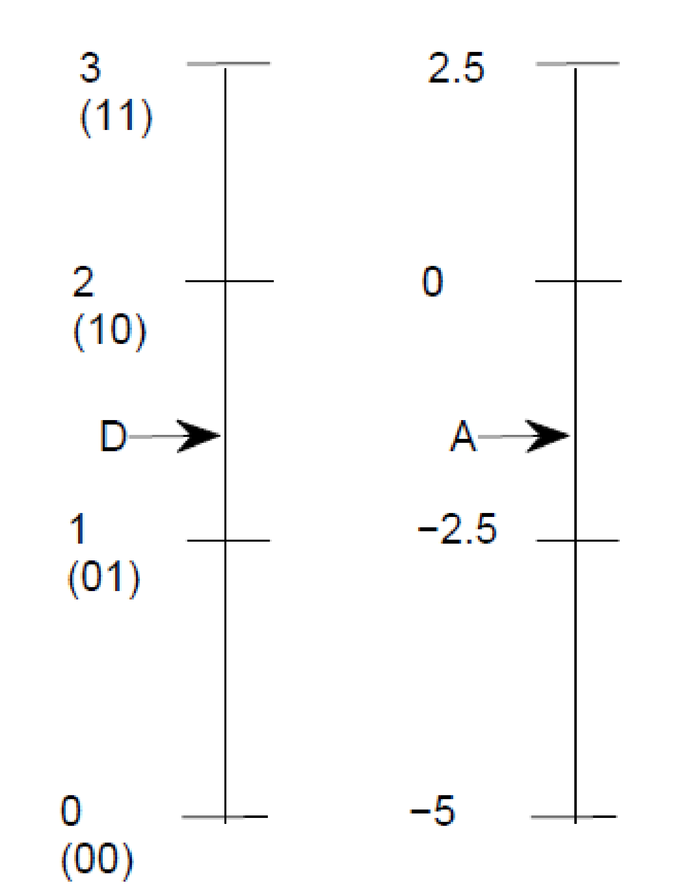
Figure C.54: Example of conversion using proportion when the dynamic ranges of both analog and digital signal are available. In this case the step size is found as $Δ = 2.5$ V and the value $A$ (or $x_{q}$ ) is related to the integer representation $D$ (or $x_{i}$ ) as $x_{q} = Δ x_{i} − 5$ .

As an example of using proportion to relate $x_{q}$ and $x_{i}$ , assume a 2-bits ADC that adopts unsigned integers as indicated in Table C.8. The task is to relate the integer codewords $x_{i} [n] ∈{0,1,2,3}$ (corresponding to 00, 01, 10 and 11, respectively) to $x_{q} [n]$ values, which can represent volts, amperes, etc. It is assumed that the original $x(t)$ is given in volts and continuously varies in the range $[−5,2.5]$ . The relation between $x_{i}$ and $x_{q}$ can be found by proportion as:

\frac{x_{i} − 0}{3 − 0} = \frac{x_{q} − (−5)}{2.5 − (−5)},

which gives

x_{q} = (\frac{7.5}{3}) x_{i} − 5 = 2.5 x_{i} − 5

and, consequently, an estimate of $Δ = 2.5$ V. In this case, the ADC associates the code 00 to $− 5$ V, 01 to $− 2.5$ V, 10 to $0$ V and 11 to $2.5$ V, as illustrated in Figure C.54. $□$

¹⁵ Lloyd’s paper is listed at [ url1qua].

¹⁶ Binary numeral systems are also discussed at [ url1bin].

¹⁷ See, e. g., [ url1flo] for more details.