Advanced: PSDs of Digitally Modulated Baseband Signals

2.11 Advanced: PSDs of Digitally Modulated Baseband Signals

The next paragraphs concern the PSDs of PAM and some line codes. Some of the results are valid for other modulations but this section focuses on baseband, linear and memoryless modulations.¹³ Modulations that use upconversion to create a passband signal are discussed in Chapter 3, which discusses QAM. Besides, most of the results are valid for linear modulations described by Eq. (2.29), but PAM is assumed for simplicity.

The model adopted here for generating a continuous-time line code is the following:

m [n] \to D/C \to m_{s} (t) \to random phase \to q_{s} (t) \to p(t) \to s (t) .

(2.24)

Basically, the PAM generation of Block (2.15) is expanded with the “random phase” from Block (A.89). Similarly, the discrete-time version of a line code can be obtained from Block (2.16) and Block (A.84).

Recall that PSDs are defined only for WSS random processes. The need for the “random phase” block is that $m_{s} (t)$ is not WSS, but wide-sense cyclostationary (WSC). In this case, its autocorrelation depends not only on the “lag” but on the absolute time too, and the PSD cannot be obtained via a Fourier transform of such bidimensional autocorrelation as for WSS processes (see Figure A.32). Randomizing the phase is a well-known procedure to transform a WSC process into a WSS, as discussed in Appendix A.19.5 without resorting to advanced mathematics.¹⁴

Block (2.24) indicates that a discrete-time signal $m [n]$ representing the symbols is converted to a sampled signal $m_{s} (t)$ and later, when the symbols are represented by $q_{s} (t)$ , they are convolved with the shaping pulse $p (t)$ to obtain the modulated signal $s (t)$ . The goal is to find an expression for the PSD $S_{s} (f)$ of $s (t)$ (or $S_{s} (e^{j Ω})$ in discrete-time).

Table 2.3 summarizes some PSD expressions for linear and memoryless baseband modulations. It can be noted that these PSDs are primarily imposed by the shaping pulse $p [n]$ (or $p (t)$ ), but the symbols also influence the spectrum via their autocorrelation $R_{m} [l]$ .

Table 2.3: Summary of PSD expressions for linear and memoryless baseband modulations.


Continuous-time (CT): general expression	$S_{s} (f) = \frac{1}{T_{sym}} \| P (f) \|^{2} \sum_{l = - \infty}^{\infty} R_{m} [l] e^{- j 2 πf T_{sym} l}$

CT for uncorrelated & zero-mean symbols	$S_{s} (f) = \frac{{\bar{E}}_{c}}{T_{sym}} \| P (f) \|^{2}$


Discrete-time (DT): general expression	$S_{s} (e^{j Ω}) = \frac{1}{L} \| P (e^{j Ω}) \|^{2} \sum_{l = - \infty}^{\infty} R_{m} [l] e^{- j Ω Ll}$

DT for uncorrelated & zero-mean symbols	$S_{s} (e^{j Ω}) = \frac{{\bar{E}}_{c}}{L} \| P (e^{j Ω}) \|^{2}$

In Table 2.3, $T_{sym}$ is the symbol interval, $P (f)$ is the Fourier transform of the shaping pulse $p (t)$ , ${\bar{E}}_{c}$ is the average constellation energy, $P (e^{j Ω})$ is the DTFT of the shaping pulse $p [n]$ and $L$ is the oversampling factor.

The general PSD expression for continuous-time in Table 2.3 correspond to using (see Section F.7.1) $S_{s} (f) = | P (f) |^{2} S_{q} (f)$ , where $P (f) = F {p (t)}$ and $S_{q} (f)$ is given by Eq. (A.92). Similarly, the discrete-time version uses Eq. (A.88).

These two PSD expressions can be simplified in the case the autocorrelation $R_{m} [l]$ of the transmit symbols is non-zero only at the origin, i. e., $R_{m} [l] = 0, l \neq 0$ . This corresponds to uncorrelated and zero-mean symbols (recall from Eq. (C.50) that $R_{m} [l] = {(𝔼 [m])}^{2}$ for $l \neq 0$ ), which lead to a white PSD. More specifically, this case leads to the simplified expressions in Table 2.3 because $R_{m} [0] = {\bar{E}}_{c}$ , where ${\bar{E}}_{c}$ is the constellation average energy given by Eq. (C.69).

As mentioned, Table 2.3 illustrates the dependence of the PSD of the transmit signal on two factors:

the spectral characteristics of the shaping pulse via $P (f)$ ;
the spectral characteristics of the pre-coded information sequence via the DTFT of $R_{m} [l]$ .

Hence there are two opportunities to control the PSD of the transmit signal.

2.11.1 Examples of PSDs

This section discusses few PSD examples. The Fourier transform of a rectangular $p (t)$ with amplitude $A$ and support $T_{sym}$ given by Eq. (A.50) is a useful result for these examples. In this case, $| P (f) |^{2} = {(A T_{sym})}^{2} {sinc}^{2} (f T_{sym})$ . When $p (t)$ is the mentioned rectangular pulse, one just needs to calculate $R_{m} [l]$ for the signal of interest. Here, the random sequence $m [n]$ is assumed to be composed by independent and equiprobable symbols. In this situation, it is interesting to contrast the case the symbols have zero-mean or not. This is done in the sequel using a polar and unipolar line codes, respectively.

Example 2.2. PSD of NRZ polar and unipolar line codes. The polar and unipolar line codes are discussed in Example A.6, where their autocorrelations are obtained. Similar procedure is repeated here. For the polar code with symbols $\pm B$ , the autocorrelation at $l = 0$ is $R_{m} [0] = {\bar{E}}_{c} = B^{2}$ . For calculating $R_{m} [1]$ , consider the product of all possible pairs of symbols: $(- B, - B), (- B, B), (B, - B), (B, B)$ , which leads to $B^{2}$ and $- B^{2}$ with probability 0.5 each. Therefore $R_{m} [1] = 0$ and, similarly, $R_{m} [l] = 0, \forall l \neq 0$ . Hence, for the NRZ pulse with amplitude $A$ and polar symbols:

S_{s} (f) = \frac{| P (f) |^{2}}{T_{sym}} \sum_{l = - \infty}^{\infty} R_{m} [l] e^{- j 2 πfl T_{sym}} = \frac{| P (f) |^{2}}{T_{sym}} R_{m} [0] e^{0} = A^{2} B^{2} T_{sym} {sinc}^{2} (f T_{sym}) .

(2.25)

For the unipolar code, $R_{m} [0] = B^{2} ∕ 2$ and averaging the products among all possible pairs $(0, 0), (0, B), (B, 0), (B, B)$ leads to $R_{m} [l] = B^{2} ∕ 4$ , for $l \neq 0$ . Hence,

\begin{align} \sum_{l = - \infty}^{\infty} R_{m} [l] e^{- j 2 πfl T_{sym}} & = \frac{B^{2}}{2} + \sum_{l = - \infty, l \neq 0}^{\infty} \frac{B^{2}}{4} e^{- j 2 πfl T_{sym}} \\ = \frac{B^{2}}{4} (1 + \sum_{l = - \infty}^{\infty} e^{- j 2 πfl T_{sym}}) \\ = \frac{B^{2}}{4} (1 + \frac{1}{T_{sym}} \sum_{k = - \infty}^{\infty} δ (f - \frac{k}{T_{sym}})) . & (2.26) \end{align}

where the last step used Eq. (A.57) and the previous one incorporated the term corresponding to $l = 0$ into the summation. When multiplying the previous expression by $| P (f) |^{2} ∕ T_{sym}$ , it should be noted that all the impulses but the one at $f = 0$ cancel with the nulls of the $sinc$ of $P (f)$ (this happens for the NRZ $p (t)$ ), leading to the PSD for the unipolar code:

S_{s} (f) = \frac{A^{2} B^{2}}{4} δ (f) + \frac{A^{2} B^{2} T_{sym}}{4} {sinc}^{2} (f T_{sym}) .

Figure 2.17 shows the PSDs of both polar and unipolar NRZ line codes for signals with power of 1 W (i.e, amplitudes 1 and $\sqrt{2}$ for polar and unipolar, respectively).

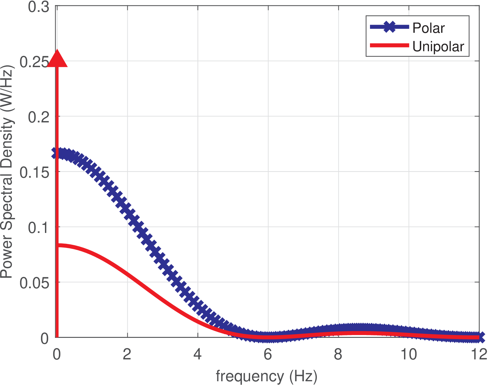
Figure 2.17: PSDs of the polar and unipolar NRZ line codes, both with signaling rate of 6 bauds and power of 1 W.

Note from Figure 2.17 that one fourth of the power of the unipolar code is concentrated at DC. Also, the only impulse for the unipolar code is at DC. The cancellation of impulses and nulls of the sinc is further discussed in Example 2.4. $□$

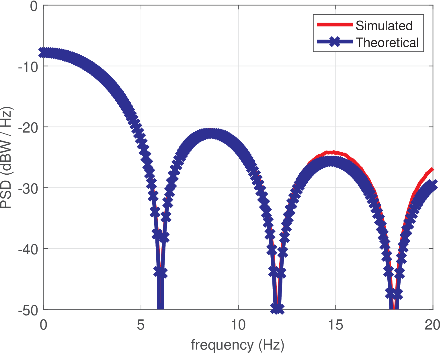
Example 2.3. Comparing theoretical and estimated PSDs of the NRZ polar code. PSD estimation techniques such as Welch’s routine, discussed in Chapter E.19, can be used for evaluating the line codes in frequency domain. Figure 2.18 compares the PSDs from the theoretical expression Eq. (2.25) and an estimation for the NRZ polar code of Figure 2.15. The results were obtained with Listing 2.13.

Figure 2.18: Comparison of estimated and theoretical PSDs for the polar NRZ line code.

Listing 2.13: MatlabOctaveCodeSnippets/snip_digi_comm_polar_psd.m

1Rb=6; %symbols (bits in this case) per second 
2Tsym=1/Rb; %symbol period 
3N=100000; %number of symbols 
4x=rand(1,N)>=0.5; %convert to 0 or 1 amplitudes 
5x=2*(x-0.5); %convert to -1 or 1 amplitudes 
6oversampling=8; %oversampling factor 
7p=ones(oversampling,1); %mimics a NRZ pulse 
8s=zeros(N*oversampling,1); %pre-allocates 
9s(1:oversampling:end)=x; %s is the upsampling of x 
10s=filter(p,1,s); %implements the convolution: s is the line code 
11window=512; %window length 
12noverlap=[]; %overlapping, [] for Octave and Matlab compatibility 
13fftsize=window; fs=oversampling*Rb; 
14%if you use below, the result is off by 3 dB: 
15%[P,f]=pwelch(s,window,noverlap,fftsize,fs,'onesided'); 
16[P,f]=pwelch(s,window,noverlap,fftsize,fs,'twosided'); 
17f=f(1:window/2); %f is from 0 to fs... 
18P=P(1:window/2); %keep only from 0 to fs/2 
19plot(f,10*log10(P),'r'); %plot the estimated PSD 
20polar=Tsym*sinc(f*Tsym).^2; % theoretical expression (A=1, B=1) 
21polardB = 10*log10(polar); hold on, plot(f,polardB,'b-x')

Note from Figure 2.18 that in this case the nulls of the sinc are at frequencies that are multiples of the symbol rate $R_{sym} = 6$ bauds, as also indicated in Figure 2.17, which uses the ordinate in linear scale (while Figure 2.18 is in logarithmic scale). $□$

Example 2.4. PSD of a RZ unipolar line code. Different from the NRZ unipolar code of Example 2.2, when the support of $p (t)$ is shorter than $T_{sym}$ (a RZ code), the impulses of the parcel in Eq. (2.26) may not be canceled by the zeros of the squared sinc of $| P (f) |^{2}$ . The current example assumes a RZ pulse $p (t)$ with amplitude $A$ and support $T_{sym} ∕ M$ from $t = - T_{sym} ∕ (2 M)$ to $T_{sym} ∕ (2 M)$ . From Eq. (A.50), the Fourier transform of $p (t)$ in this case is $P (f) = (A T_{sym} ∕ M) sinc (f T_{sym} ∕ M)$ with nulls at frequencies multiple of $M ∕ T_{sym}$ while Eq. (2.26) has impulses spaced by $1 ∕ T_{sym}$ . Combining $| P (f) |^{2} ∕ T_{sym}$ with Eq. (2.26) leads to the following PSD for the RZ unipolar:

S_{s} (f) = \frac{A^{2} B^{2} T_{sym}}{4 M^{2}} {sinc}^{2} (\frac{f T_{sym}}{M}) [1 + \frac{1}{T_{sym}} \sum_{k = - \infty}^{\infty} δ (f - \frac{k}{T_{sym}})] .

(2.27)

In this case, the PSD presents the impulses of Eq. (2.26) that are not located at frequencies multiple of $M R_{sym}$ . Figure 2.19 presents Eq. (2.27) for $A = B = 1$ , $R_{sym} = 6$ bauds and $M = 4$ , superimposed to the estimated PSD.

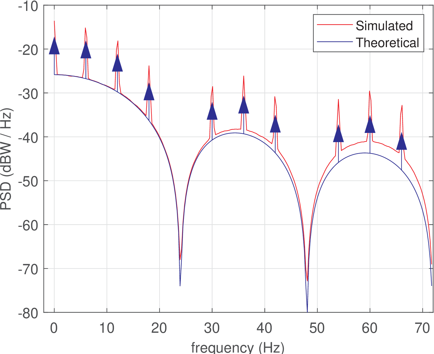
Figure 2.19: PSD of RZ unipolar code with symbol interval $T_{sym} = 1 ∕ 6$ s and shaping pulse with support $T_{sym} ∕ 4$ .

Note in Figure 2.19 that the peaks of the estimated PSD coincide with the impulses, but not with their areas. This is expected given that the infinite amplitude of the impulses is not realizable. Besides, the PSD value depends on the FFT bin width used in the estimation process. To highlight this dependence, Figure 2.20 was obtained with a PSD estimated via the same procedure that generated Figure 2.19 but with a smaller FFT bin width (1024 times smaller, which corresponds to $10 {log}_{10} 1024 \approx 30$ dB).

Figure 2.20: PSD of RZ unipolar code estimated with smaller FFT bin width than Figure 2.19.

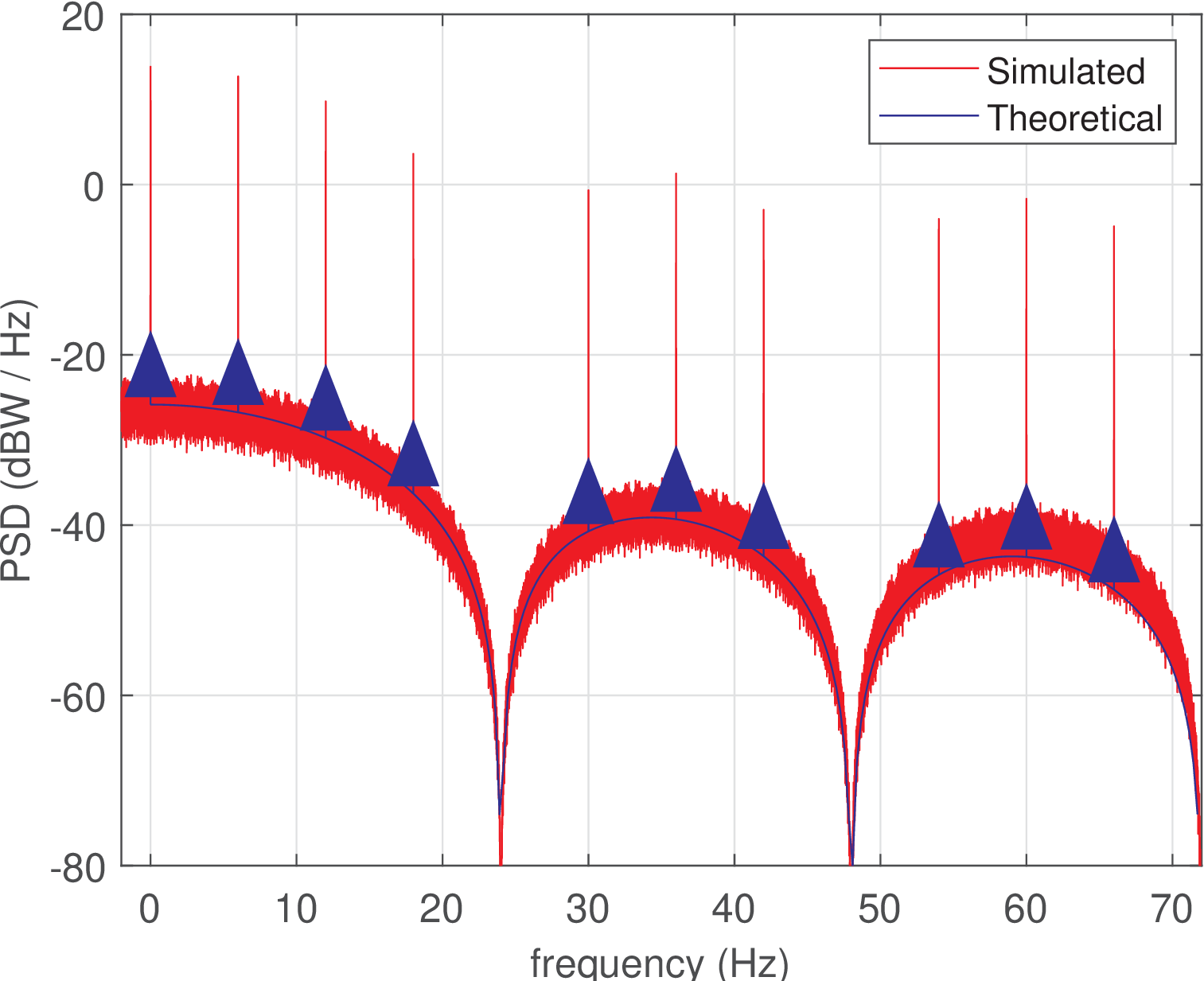
Comparing Figure 2.19 and Figure 2.20, it can be seen that the PSD peaks corresponding to impulses increased by approximately 30 dB while the variance of the estimated PSD also increased significantly. This issue is discussed in Chapter E.19. $□$

Example 2.5. Comparing theoretical and estimated PSDs of a PAM signal. A typical PAM constellation obeys the guidelines listed in Section 2.7.1. Consequently, the uncorrelated and zero-mean symbols lead to an autocorrelation that is non-zero only at lag $l = 0$ , with this value $R [0] = {\bar{E}}_{c}$ coinciding with the constellation average energy. Hence, from Table 2.3, the PSD for such PAMs is

S_{s} (f) = \frac{{\bar{E}}_{c}}{T_{sym}} | P (f) |^{2} .

(2.28)

Listing 2.14 compares a theoretical curve for the PSD of a discrete-time PAM signal and an estimated PSD.

Listing 2.14: MatlabOctaveCodeSnippets/snip_digi_comm_PAM_PSD.m

1M=16; %modulation order, number of distinct symbols 
2N = 400000; % number of symbols 
3L=8; %oversampling factor 
4indices=floor(M*rand(1,N))+1; %random indices from [1, M] 
5alphabet=[-(M-1):2:M-1]; %symbols ...,-3,-1,1,3,5,7,... 
6Ec=mean(alphabet.^2); %constellation average energy 
7symbols=alphabet(indices); %obtain M random symbols 
8m_upsampled=zeros(1,N*L); %pre-allocate space with zeros 
9m_upsampled(1:L:end)=symbols; %insert symbols, L-1 zeros in-between 
10p=ones(1,L); %shaping pulse is a NRZ square waveform 
11s=conv(m_upsampled,p); %convolve symbols with shaping pulse 
12Fs = 2*pi; %normalized sampling frequency 
13[SpamEstimated,f]=ak_psd(s,Fs); %find PSD in dBm/Hz 
14Tsym=L/Fs; %the normalized symbol interval 
15SpamTheoretical=Ec*Tsym*sinc(f*Tsym).^2; % theoretical expression 
16clf; plot(f,SpamEstimated-30,f,10*log10(SpamTheoretical),'.-r'); 
17xlabel('\Omega (rad)'); ylabel('PSD (dBW / normalized freq.)'); 
18legend('Estimated','Theoretical'), axis([-pi pi -20 30]), grid

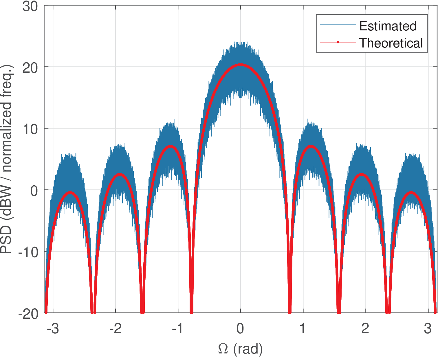
Figure 2.21: Comparison of theoretical and estimated curves for the PSD of a 16-PAM discrete-time signal with oversampling $L = 8$ .

Figure 2.21 confirms that the modulation order $M$ of a PAM simply scales the PSD via ${\bar{E}}_{c}$ , while the PSD shape (number of nulls, etc.) is imposed by the pulse $p (t)$ . $□$

Example 2.6. PSDs of binary ASK, FSK and PSK. The PSDs of ASK, FSK and PSK can be obtained from frequency upconversion of their corresponding baseband signals. This fact is discussed in this example.

Figure 2.22 illustrates the PSDs of all three modulations. The time-domain signals were obtained with ak_simpleBinaryModulation.m using a symbol rate of $R_{sym} = 500$ bauds.

Figure 2.22: PSDs for the given binary ASK, FSK and PSK.

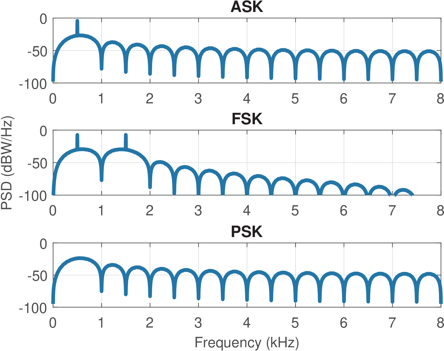
In Figure 2.22, there are peaks at 500 Hz for ASK, 500 and 1500 for FSK and no peak for PSK. All these peaks correspond to impulses in the theoretical expressions (see Figure 2.17). Note that ASK and PSK are obtained from baseband unipolar and polar (NRZ) line codes. Similarly, the FSK can be seen as the sum of two unipolar signals that were previously multiplied by distinct carrier frequencies. Therefore, a PSK does not have an impulse in its PSD because it corresponds to an upconverted version of the NRZ polar. In contrast, ASK has one impulse at the carrier frequency and FSK has two impulses positioned at the respective two frequencies. This fact is emphasized in Figure 2.23 for PAM and ASK, in which ASK was generated by multiplying the PAM by a carrier with frequency $f_{c} \approx 4.17$ Hz. In practice, due to the finite duration of the simulated signals, the theoretical ASK impulse shows up as a peak at $f_{c} \approx 4.17$ Hz in the ASK PSD.

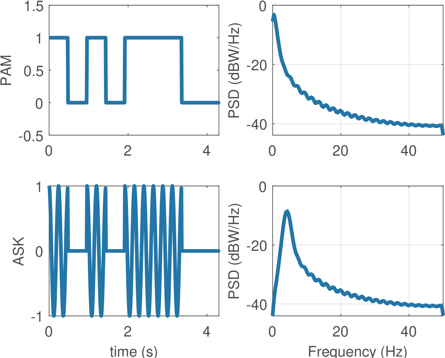
Figure 2.23: Binary baseband PAM and its corresponding passband ASK signal. The left plots are the waveforms and the right plots their PSDs.

Figure 2.23 provides an example where the bitstream is [1 0 1 0 1 1 1 0]. The PAM uses oversampling $L = 48$ and $F_{s} = 100$ Hz. The ASK uses a carrier at $Ω_{c} = 2 π ∕ 24$ rad, which corresponds to $f_{c} = F_{s} ∕ 24 \approx 4.17$ Hz. The PSDs were estimated with low frequency resolution but the effect of frequency upconversion can be easily noted. $□$

¹³ Calculating the PSD of line codes that use memory is more involved and can be studied in digital communication textbooks such as [PS07] or [Pee86].

¹⁴ Appendix A.19.3 can be used to improve understanding about cyclostationarity but Appendix A.19.5 suffices for the purposes here.