2.13 Simple example of M-PAM simulation over AWGN
This section starts by analyzing M-PAM transmission over AWGN using a simulation on Matlab/Octave. The reader is encouraged to run and understand the simulation before proceeding.
The function ak_waveformSimulationOfPAMInAWGN.m listed below presents a simple PAM simulation. The channel simply adds Gaussian noise (no filtering, the channel impulse response is ) and the receiver makes its decision based on a single sample, arbitrarily extracted from the middle of each symbol interval.
1function [ber,ser,SNRdB] = ...
2    ak_waveformSimulationOfPAMInAWGN(numberOfBytes,...
3    oversample, M, noisePower)
4%[ber,ser,SNRdB] = ...
5%    ak_waveformSimulationOfPAMInAWGN(numberOfBytes,...
6%    oversample, M, noisePower)
7%Inputs:
8%numberOfBytes -> number of bytes to be transmitted
9%oversample -> oversampling factor
10%M -> modulation order (number of constellation symbols)
11%noisePower -> noise power
12%Outputs:
13%ber -> bit error rate
14%ser -> symbol error rate
15%SNRdB -> signal to noise ratio in dB
16b=log2(M); %number of bits per symbol
17bytesTx = floor(256*rand(1,numberOfBytes)); %random bytes
18symbolIndicesTx = ak_sliceBytes(bytesTx, b);
19%constellation = pammod(0:M-1, M); %see the constelllation
20symbols = pammod(symbolIndicesTx,M); % modulate
21%% 1) Convert symbols into a waveform:
22p = ones(1,oversample); %define a simple shaping pulse
23p = p / (mean(p.^2)); %make sure pulse has unitary power
24numSymbols = length(symbols); %number of symbols
25waveform = zeros(1,numSymbols*oversample); %pre-allocate
26waveform(1:oversample:end) = symbols;
27waveform = filter(p,1,waveform); % Pulse shaping filtering
28%% 2) Send waveform through AWGN channel
29n = sqrt(noisePower)*randn(size(waveform));%generate noise
30r = waveform + n; %add transmitted signal and noise
31SNRdB=10*log10(mean(waveform.^2)/mean(n.^2));%estimate SNR
32%% 3) Implement simple receiver:
33initialSample = oversample/2; %sample in middle of symbol
34receivedSymbols = r(initialSample:oversample:end); %sample
35symbolIndicesRx = pamdemod(receivedSymbols, M);
36bytesRx = ak_unsliceBytes(symbolIndicesRx, b);
37ser = ak_calculateSymbolErrorRate(symbolIndicesTx, ...
38    symbolIndicesRx); %estimate SER
39ber = ak_estimateBERFromBytes(bytesTx, bytesRx); % BER
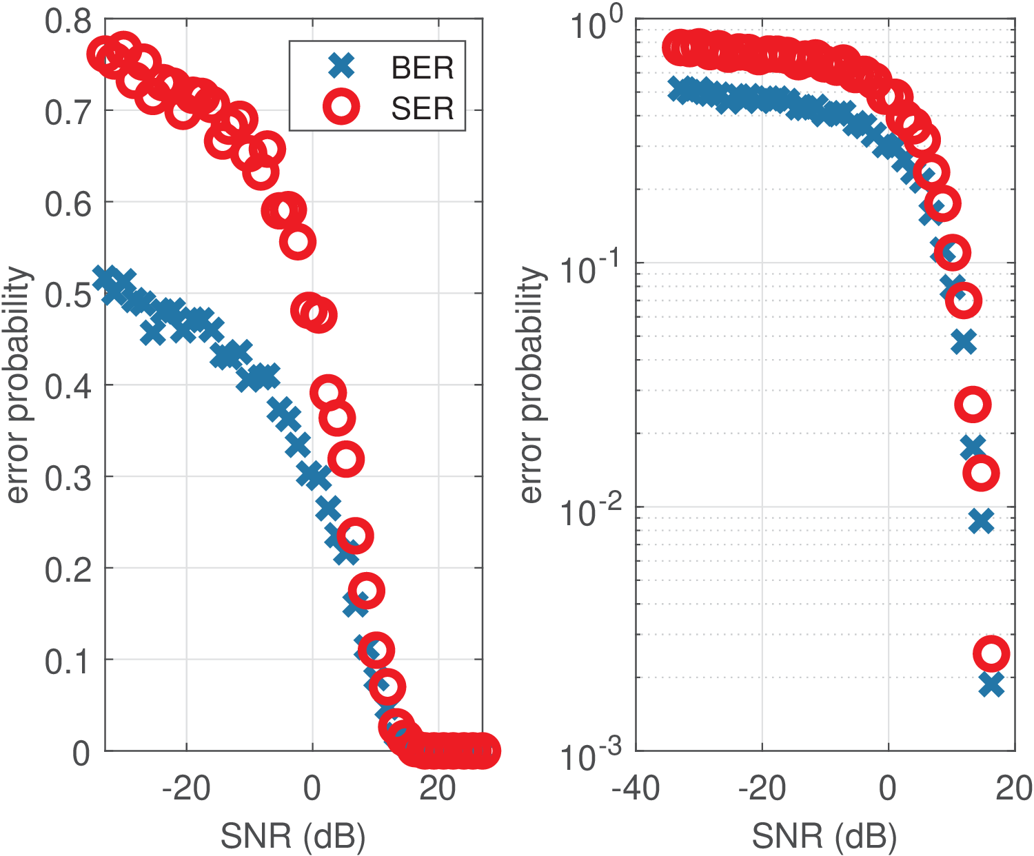
Using this code and varying the noise power, the error probabilities in Figure 2.27 are obtained.
In Figure 2.27, the plot at the right is a version using semilogy.m of the one at the left. Note that Matlab/Octave cannot show the log of 0 and the right abscissa is smaller than the left one because there are zero errors for SNR larger than approximately 17 dB. To reliably estimate the SER for larger SNR, the number of transmitted symbols would have to be increased.