Applications

3.14 Applications

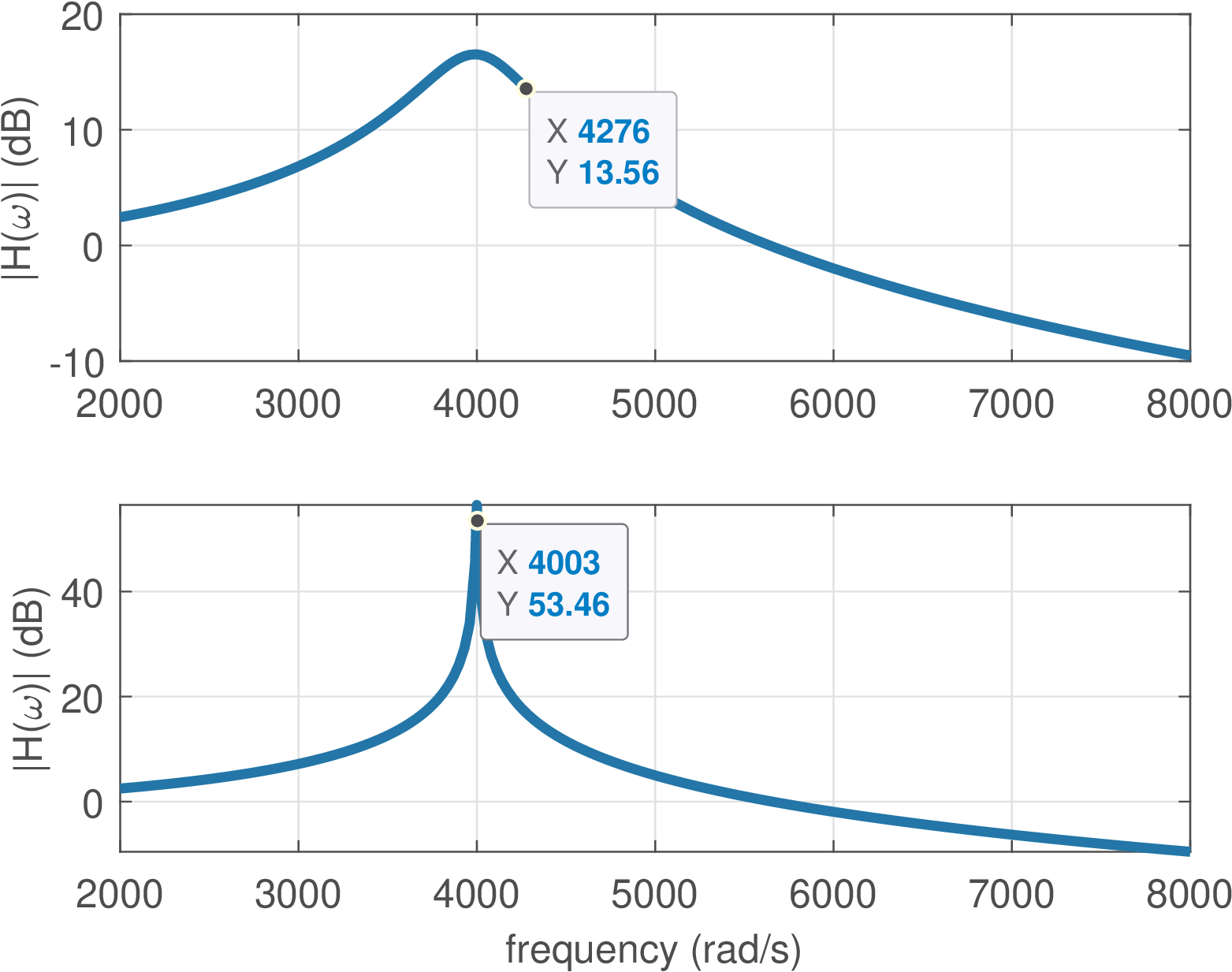
Application 3.1. Influence of the poles quality factor on frequency response. The goal here is to illustrate how the pole Q-factor influences a frequency response.

Figure 3.74: Magnitudes of frequency responses for two resonators with $H (s)$ as in Eq. (3.17). The top plot corresponds to poles $p = - 300 \pm j 4000$ with $Q \approx 6.6854$ and $| H (ω) |_{ω = 4000} = 16.52$ dB. The bottom plot corresponds to $p = - 3 \pm j 4000$ with $Q \approx 666.67$ and $| H (ω) |_{ω = 4000} = 56.48$ dB. The two data tips indicate approximately 3-dB frequencies.

First, Listing 3.38 shows how to calculate $Q$ for a second-order system in Matlab/Octave using Eq. (3.28).

Listing 3.38: MatlabOctaveCodeSnippets/snip_systems_Qfactor.m. [ Python version]

1p1=-300+j*4000; p2=-300-j*4000; %pole and its conjugate 
2A=poly([p1 p2]); %convert it to a polynomial A(s) 
3omega_n = sqrt(A(3)); alpha = A(2)/2; %use definitions 
4Q = omega_n / (2*alpha) %calculate Q-factor

In this case, the poles are located at the frequency $\pm 4000$ rad/s and have $Q \approx 6.6854$ . For this example, the 3-dB bandwidth is defined (approximately) by $ω_{1} = 3678$ and $ω_{2} = 4276.3$ rad/s, which gives $BW = (ω_{2} - ω_{1}) ∕ (2 π) \approx 95.2$ Hz. If we change the poles to $- 3 \pm j 4000$ , the $Q$ -factor increases to $Q \approx 666.67$ and $BW$ decreases to approximately 6 Hz. Figure 3.74 compares these two situations.

The approximations used in analog filter design differ in the strategy for locating the poles (and zeros). Typically, the approximations that use poles with larger $Q$ -factor have better magnitude but worse phase responses. The Listing 3.39 compares the poles and their $Q$ values for the Butterworth, Chebyshev (Type 1) and Cauer (or elliptic), which are listed in Table 3.8.

Listing 3.39: MatlabOctaveFunctions/ak_showQfactors.m

1function ak_showQfactors 
2N=6; %order of filter 
3Wc=100; %cutoff frequency 
4disp('- Butterworth filter:'); 
5[z,p,k]=butter(N,Wc,'s'); %design Butterworth 
6calculateQfactors(p) %calculate and display Q-factors 
7disp('- Chebyshev 1 filter:'); 
8Rp=1; %maximum ripple at passband 
9[z,p,k]=cheby1(N,Rp,Wc,'s'); %design Chebyshev type 1 
10calculateQfactors(p) %calculate and display Q-factors 
11disp('- Elliptic filter:'); 
12Rs=30; %minimum attenuation at stopband 
13Wp=Wc; %elliptic natural frequency equals cutoff frequency 
14[z,p,k]=ellip(N,Rp,Rs,Wp,'s'); %design Elliptic filter 
15calculateQfactors(p) %calculate and display Q-factors 
16end % end function ak_showQfactors 
17function calculateQfactors(p) %p has the poles 
18p=p(find(imag(p)>0)); %exclude real poles and complex conjugates 
19N=length(p); %number of complex poles with non-zero imaginary parts 
20for i=1:2:N 
21    pole = p(i); 
22    Q = abs(pole) / (2*(-real(pole))); 
23    disp(['Poles=' num2str(real(pole)) ' +/- j' ... 
24        num2str(imag(pole)) ' => Q=' num2str(Q)]); 
25end %end for 
26end %end function calculateQfactors

The output of Listing 3.39 is the following:

- Butterworth filter:
Poles=-96.5926 +/- j25.8819 => Q=0.51764
Poles=-70.7107 +/- j70.7107 => Q=0.70711
Poles=-25.8819 +/- j96.5926 => Q=1.9319
- Chebyshev 1 filter:
Poles=-23.2063 +/- j26.6184 => Q=0.76087
Poles=-16.9882 +/- j72.7227 => Q=2.198
Poles=-6.2181 +/- j99.3411 => Q=8.0037
- Elliptic filter:
Poles=-34.9934 +/- j49.0885 => Q=0.86137
Poles=-9.154 +/- j92.2792 => Q=5.0651
Poles=-1.3808 +/- j100.0259 => Q=36.2244

These results indicate that elliptic filters are more aggressive with respect to pole positioning (the poles are closer to the $jω$ axis) and have sharper magnitude responses. Butterworth filters, on the other hand, have poles with lower $Q$ than Chebyshev and elliptic filters.

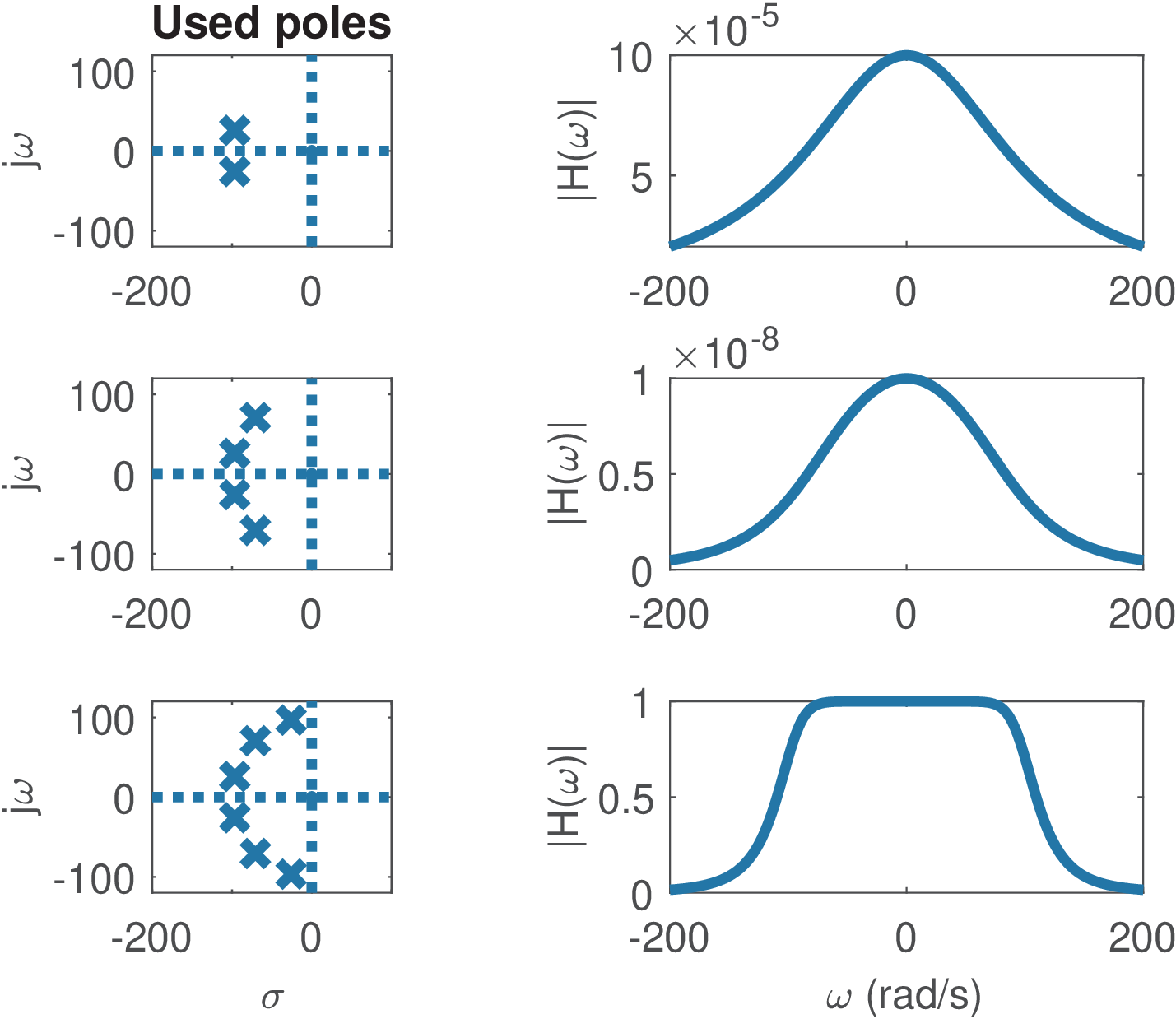
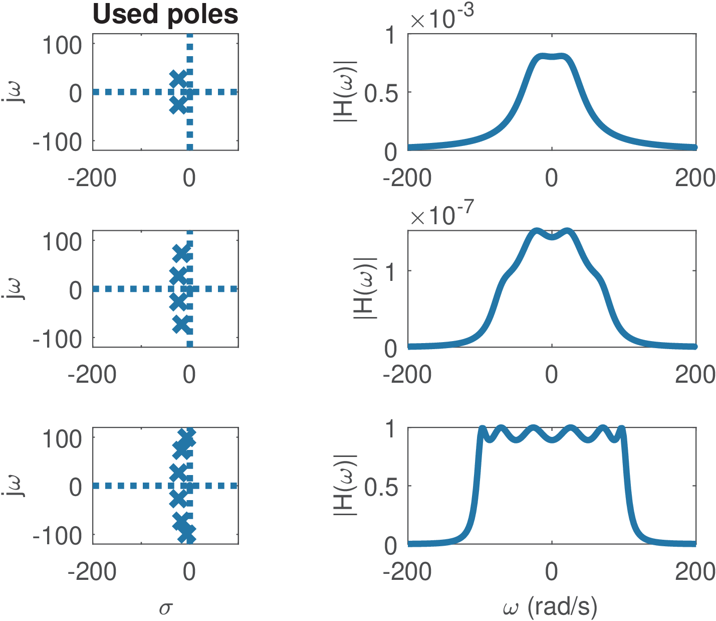
Figure 3.75: Poles (left) and magnitude $| H (ω) |$ (right) for the sixth-order Butterworth filter of Listing 3.39. The top plots are obtained with the pair of poles with the smallest $Q$ , the middle plots with four poles and the bottom plots with all six poles.

Figure 3.76: Similar to Figure 3.75, but with a sixth-order Chebyshev Type 1 filter. Note the poles are closer to the $jω$ axis than for the Butterworth filter and there are ripples in the passband (one peak for each pole).

Figure 3.75 and Figure 3.76 compare the Butterworth and Chebyshev approximations using sixth-order filters. Both lead to all-poles transfer functions, because there are no finite zeros (all zeros are at $ω = \pm \infty$ ). Finite zeros offer an additional degree of freedom but typically create additional abrupt changes in phase.

Figure 3.77: Zero-pole plot (top) and magnitude in dB (bottom) for the sixth-order elliptic filter of Listing 3.39. This filter has zeros at $ω = \pm 104.6303$ , $\pm 116.8868$ , $\pm 242.7541$ rad/s, each one imposing a “valley” in the magnitude response, as the one indicated for $ω = 104.6303$ .

The elliptic filters use finite zeros and achieve very short transition regions. Figure 3.77 illustrates a sixth-order elliptic filter to be compared to Figure 3.75 and Figure 3.76 (their bottom-most plots). $□$

Application 3.2. Understanding and compensating the delay imposed by a system. All practical systems impose some delay or distortion to signals. For example, in communication systems the channel is typically frequency-selective, meaning that distinct frequency components of the signal get attenuated and delayed in a way that the output signal is a distorted version of the input signal. Besides this effect, systems impose a delay (the output is observed only after an interval of time from the instant the input was generated, as studied in Application 1.1) that is often characterized by its group-delay. Better understanding how to predict this delay when the system is LTI is the subject of the following discussion.

An example of filtering is provided in the sequel using an 8-th order IIR filter obtained and analyzed with Listing 3.40.

Listing 3.40: MatlabOctaveCodeSnippets/snip_systems_filtering.m. [ Python version]

1[B,A]=butter(8,0.3); %IIR filter 
2h=impz(B,A,50); %obtain h[n], truncated in 50 samples 
3grpdelay(B,A); %plots the group delay of the filter 
4x=[1:20,20:-1:1]; %input signal to be filtered, in Volts 
5X=fft(x)/length(x); %FFT of x, to be read in Volts 
6y=conv(x,h); %convolution y=x*h

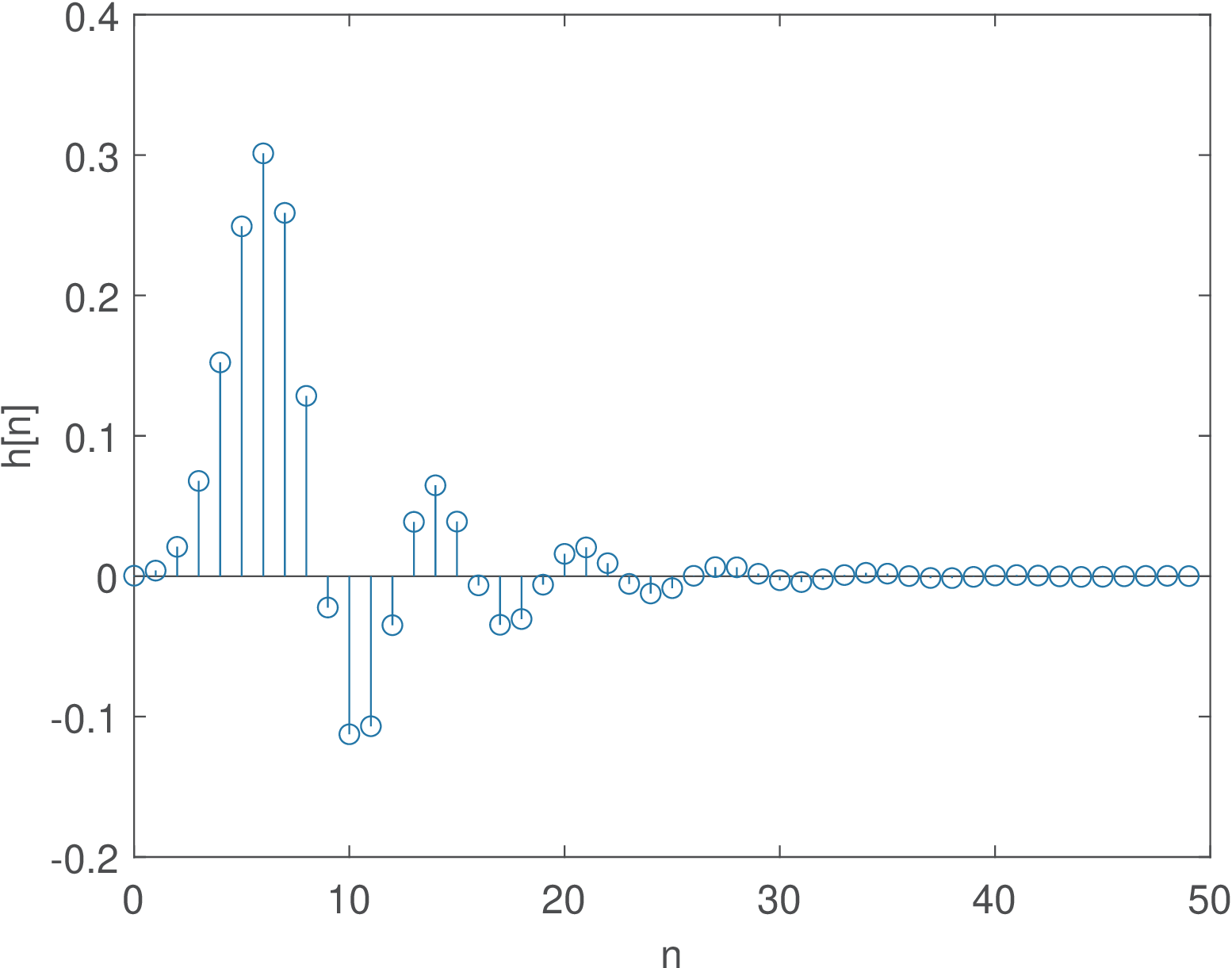
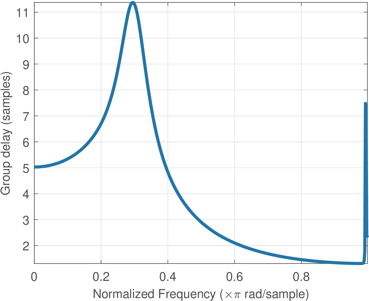
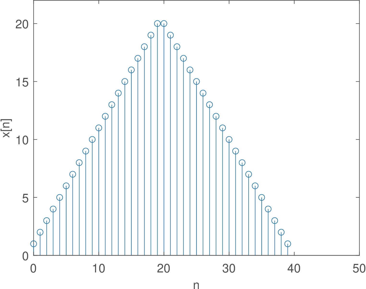
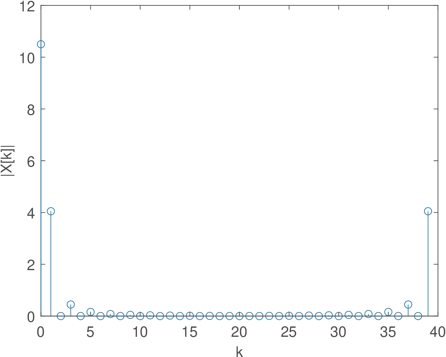
The truncated impulse response of this filter is depicted in Figure 3.77a and the group delay in Figure 3.77b. An input signal x with a triangular shape was generated and is depicted in Figure 3.79 together with its FFT.

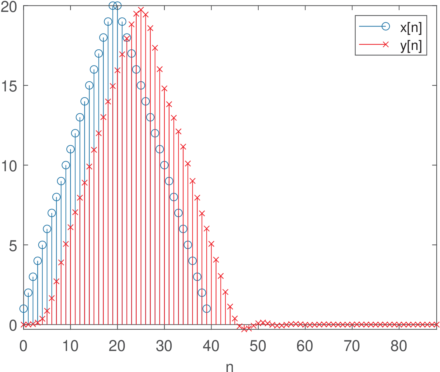
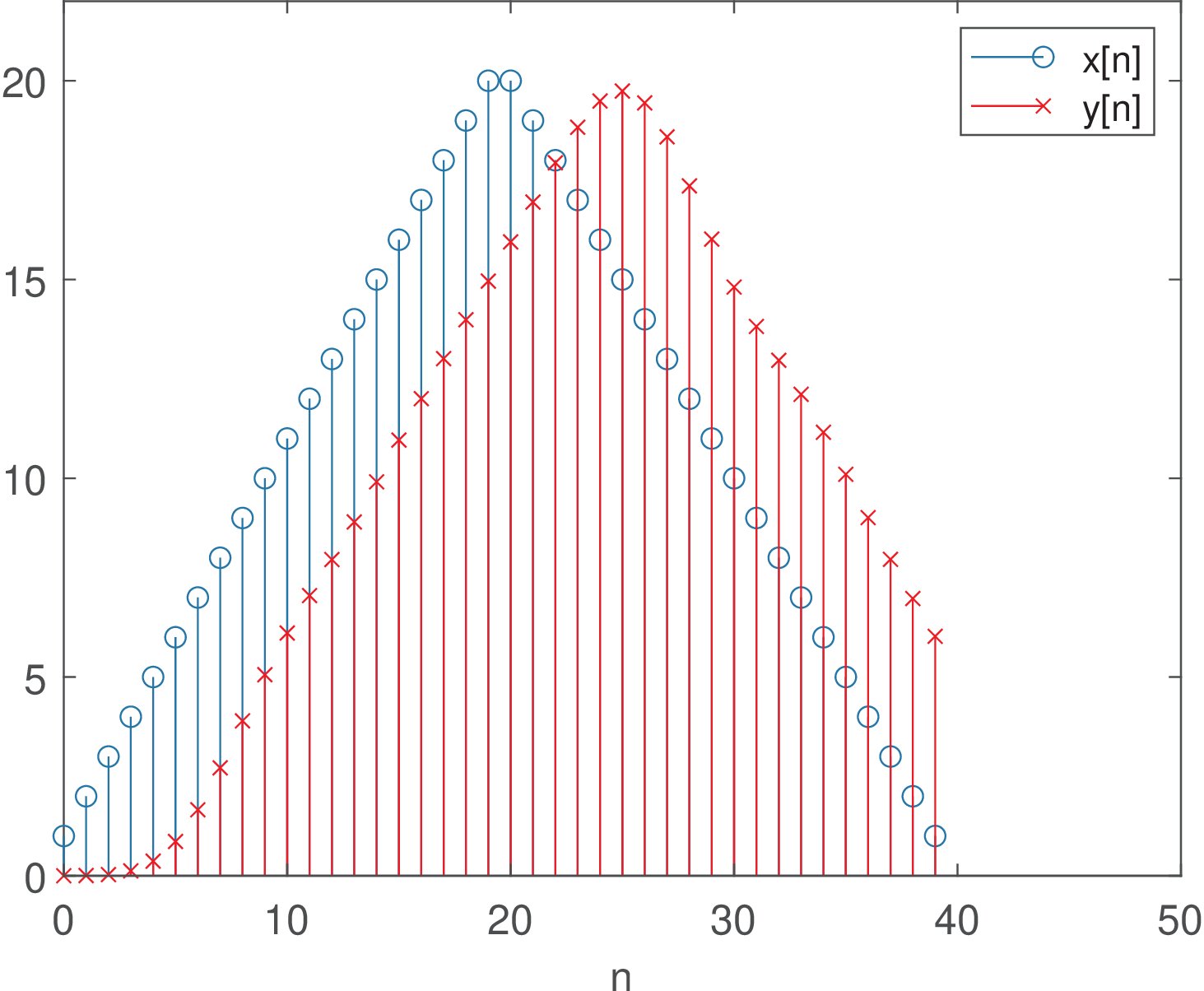
Figure 3.80: Input $x [n]$ and output $y [n]$ signals obtained via convolution with truncated $h [n]$ .

The result of the convolution y=conv(x,h) is shown in Figure 3.80. The input has peaks at $n = 19$ and $n = 20$ , such that x[19]=x[20]=20, while the output peaked at $n = 25$ with y[25]=19.7. This delay of 5 samples could be inferred by observing that the peak of h in Figure 3.77a is located at sample $n = 6$ . A more accurate analysis can be done via the filter’s group delay. In the case of a linear-phase FIR, the group delay is constant (the same number of samples) in the whole passband. But the current IIR has a frequency dependent group delay and the spectrum of the input signal needs to be analyzed via Figure 3.79.

Note that most of the input signal power is concentrated at DC and the FFT coefficient $X [k]$ for $k = 1$ , which corresponds to an angle $Ω = 2 π ∕ 40 = 0.1571$ rad, given that length(x)=40 is the FFT length. From Figure 3.77b or directly calculating gd=grpdelay(B,A,[0 0.1571]), it can be observed that the group delay $τ_{g} (Ω)$ of the filter for components at $k = 0$ and $k = 1$ is $τ_{g} (0) = 5.03$ and $τ_{g} (0.1571) = 5.1043$ samples, respectively. When using Figure 3.77b, note that $Ω$ should be normalized and the value read at $Ω ∕ π = 0.05$ . The group delay at the frequencies of interest is approximately 5 samples, which explains the delay imposed by the filter in Figure 3.80.

Figure 3.81: Input $x [n]$ and output $y [n]$ signals obtained via filter.

Instead of using convolution, the output was obtained with y=filter(B,A,x). In this case, the vector y is the one depicted in Figure 3.81, which should be compared to Figure 3.80. Because $N_{x} = 40$ and $N_{h} = 50$ samples, the convolution in Figure 3.80 led to $N_{y} = 40 + 50 - 1 = 89$ samples. In contrast, Figure 3.81 shows that filter makes sure that $N_{y} = N_{x} = 40$ samples. To visualize the tail of the convolution, one should add zero samples to the end of x. For example, the extra 20 samples in y=filter(B,A,[x zeros(1,20)]) are enough to visualize the “triangle” in y.

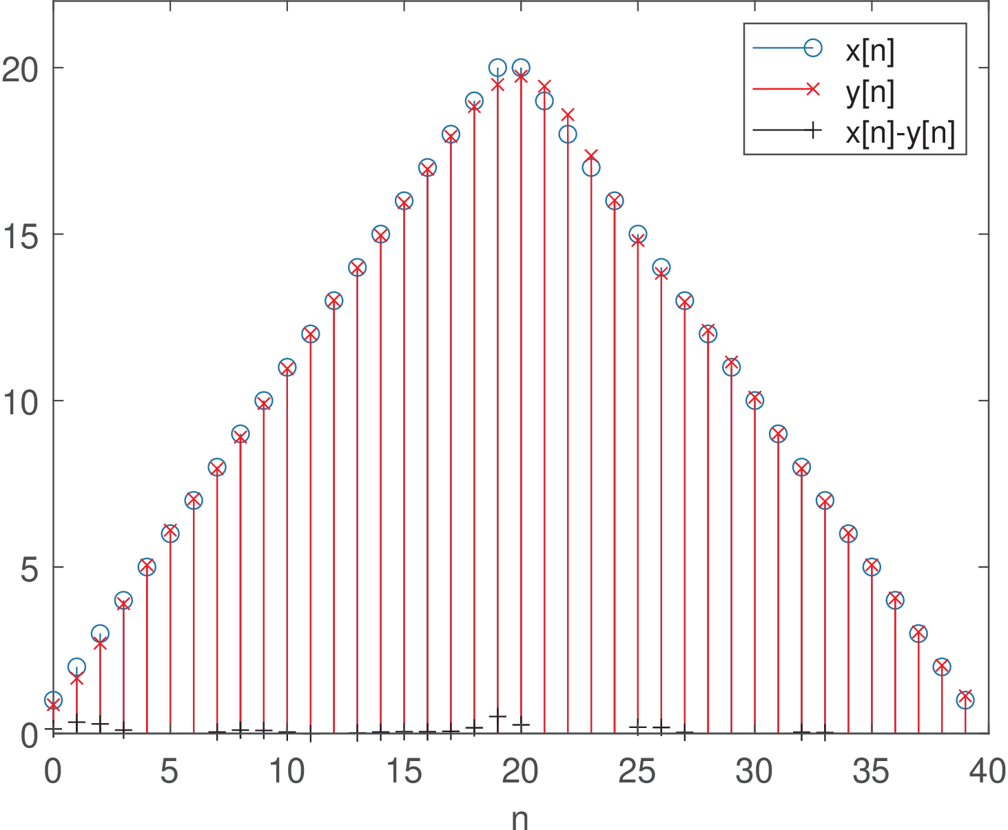
Figure 3.82: Output $y [n]$ aligned with the input $x [n]$ and corresponding error $x [n] - y [n]$ .

In some situations it is necessary to compare the error between the input and filtered output signals. But this requires compensating the filter delay and eliminating the convolution tail. Figure 3.82 was obtained with:

Listing 3.41: MatlabOctaveCodeSnippets/snip_systems_compensate_grpdelay.m. [ Python version]

1x=[1:20,20:-1:1]; %input signal to be filtered, in Volts 
2[B,A]=butter(8,0.3); %IIR filter 
3h=impz(B,A,50); %truncate h[n] using 50 samples 
4y=conv(x,h);  %convolution y=x*h 
5x=x(:); y=y(:); %force both x and y to be column vectors 
6meanGroupDelay=5 %estimated "best" filter delay 
7y(1:meanGroupDelay)=[]; %compensate the filter delay 
8y(length(x)+1:end)=[]; %eliminate convolution tail 
9mse=mean( (x-y).^2 ) %calculate the mean squared error 
10SNR=10*log10(mean(x.^2)/mse) %estimate signal/noise ratio 
11stem(0:length(x)-1,x); hold on %input 
12stem(0:length(y)-1,y,'r') %output aligned with the input 
13stem(0:length(y)-1,x-y,'k') %e.g., calculate error after alignment

The mean squared error (MSE) in this case is 0.0363, which is equivalent to an SNR of 35.97 dB.

Decreasing the filter cutoff frequency to $Ω = 0.1$ rad via [B,A]=butter(8,0.1) and adjusting the variable meanGroupDelay to 16 samples (meanGroupDelay=17 leads to a slightly better result) makes the SNR decrease to 23.22 dB because more high frequency components of x are filtered out. $□$

Application 3.3. Taking the filter memory in account. When using filter in block processing, it is important to take the filter’s memory in account. By default, this memory is assumed to be zero (the system is relaxed), but this can be modified with the command filtic, which allows to set the filter’s initial conditions.

Figure 3.83: Filtering in blocks of $N = 5$ samples but not updating the filter’s memory.

Instead of using y=filter(B,A,x) to completely filter x in one function call, it is useful to know how to segment the input x in blocks of $N$ samples and repeatedly invoke filter until filtering all blocks. This is illustrated in Listing 3.42.

Listing 3.42: MatlabOctaveCodeSnippets/snip_systems_filtering_blocks.m. [ Python version]

1x=[1:20,20:-1:1]; %input signal to be filtered, in Volts 
2[B,A]=butter(8,0.3); %IIR filter 
3N=5; %block length 
4numBlocks=floor(length(x)/N); %number of blocks 
5Zi=filtic(B,A,0); %initialize the filter memory with zero samples 
6y=zeros(size(x)); %pre-allocate space for the output 
7for i=0:numBlocks-1 
8    startSample = i*N + 1; %begin of current block 
9    endSample = startSample+N -1; %end of current block 
10    xb=x(startSample:endSample); %extract current block 
11    [yb,Zi]=filter(B,A,xb,Zi);%filter and update memory 
12    y(startSample:endSample)=yb; %update vector y 
13end

These commands obtain the same results of Figure 3.81 because the filter memory is updated via [yb,Zi]=filter(B,A,xb,Zi). However, a simple modification from this command to yb=filter(B,A,xb), which disregards the filter memory leads to the result in Figure 3.83. In this case, the filter has zeroed memory at the beginning of each block of $N = 5$ samples. The strong distortion on $y [n]$ in this case indicates that it is crucial to take care of updating the filter memory when dealing with signal processing in blocks. $□$

Application 3.4. Processing sample blocks using convolution in matrix notation.

As Eq. (3.16) indicates, the convolution between two finite-length signals can be represented in matrix notation. However, in many applications, block processing is adopted, where one of the signals has an infinite duration and is segmented into successive blocks of $N$ samples, as in Eq. (1.9).

Listing 3.43 illustrates the extra manipulations that are required to use a matrix notation for the convolution of each block and get the correct convolution result.

Listing 3.43: MatlabOctaveCodeSnippets/snip_systems_matrixBlockConvolutions.m. [ Python version]

1x=transpose(1:1000); %(eventually long) input signal,as column vector 
2h=ones(3,1); %non-zero samples of finite-length impulse response 
3Nh=length(h); %number of impulse response non-zero samples 
4Nb=5; %block (segment) length 
5Nbout = Nb+Nh-1; %number of samples at the output of each block 
6Nx = length(x); %number of input samples 
7hmatrix = convmtx(h,Nb); %impulse resp. in matrix notation 
8beginNdx = 1; %initialize index for first sample of current block 
9y = zeros(Nh+Nx-1,1); %pre-allocate space for convolution output 
10for beginNdx=1:Nb:Nx %loop over all blocks 
11    endIndex = beginNdx+Nb-1; %current block end index 
12    xblock=x(beginNdx:endIndex); %block samples, as column vector 
13    yblock = hmatrix * xblock; %perform convolution for this block 
14    y(beginNdx:beginNdx+Nbout-1) = y(beginNdx:beginNdx+Nbout-1) + ... 
15        yblock; %add parcial result 
16end 
17plot(y-conv(x,h)) %compare the error with result from conv

The basic idea is that the end samples (“tails”) of the partial convolution results need to be properly added to the final result. In the example of Listing 3.43, the impulse response has Nh=3 non-zero samples and the block length is Nb=5. The convolution matrix hmatrix has dimension $7 \times 5$ and each partial convolution result corresponds to Nbout=7 samples. For instance, the last two samples of yblock of the first block need to be added to the first two samples of yblock obtained of the second block, and so on. This is similar to the overlap-add method illustrated in Listing 3.5 but without the FFT-based processing. $□$

Application 3.5. Power and energy at the output of a LTI system. In many applications it is important to estimate the power at the output of a system. The following result is valid for LTI systems.

Theorem 3. Power at the output of a discrete-time LTI system.

P_{y} = P_{x} E_{h} + 2 \sum_{i = 0}^{L} ∑_{j = 0, j \neq i}^{L} h_{i} h_{j} R_{x} (j - i)

(3.109)

where $R_{x} (j - i) = 𝔼 [⟨ x [n], x [n - (j - i)] ⟩]$ is the empirical (time-averaged) autocorrelation and $E_{h} = \sum_{i = 0}^{L} h_{i}^{2}$ is the energy of $h [n]$ . If $R_{x} (k) = 0, \forall k$ and $k \neq 0$ , then $P_{y} = P_{x} E_{h}$ .

Proof sketch: Assume a short impulse response $h [n] = h_{0} + h_{1} δ [n - 1] + h_{2} δ [n - 2]$ with $L = 2$ . Take three consecutive output values starting at an arbitrary time instant, such as $n = 5$ , for example. These values will be $y [5] = x [5] h_{0} + x [4] h_{1} + x [3] h_{2}$ , $y [6] = x [6] h_{0} + x [5] h_{1} + x [4] h_{2}$ and $y [7] = x [7] h_{0} + x [6] h_{1} + x [5] h_{2}$ . Calculating the energy $E_{y}$ for these three samples is enough to provide insight on the solution:

\begin{array}{l} E_{y} & = y^{2} [5] + y^{2} [6] + y^{2} [7] \\ = h_{0}^{2} (x^{2} [5] + x^{2} [6] + x^{2} [7]) + h_{1}^{2} (x^{2} [4] + x^{2} [5] + x^{2} [6]) \\ + h_{2}^{2} (x^{2} [3] + x^{2} [4] + x^{2} [5]) + 2 h_{0} h_{1} (x [5] x [4] + x [6] x [5] + x [7] x [6]) \\ + 2 h_{0} h_{2} (x [5] x [3] + x [6] x [4] + x [7] x [5]) \\ + 2 h_{1} h_{2} (x [4] x [3] + x [5] x [4] + x [6] x [5]) . \end{array}

Taking all samples in account and using expectation, one can obtain a relation between the output and input energies $E_{y}$ and $E_{x}$ , respectively:

E_{y} = E_{x} E_{h} + 2 \sum_{i = 0}^{L} ∑_{j = 0, j \neq i}^{L} h_{i} h_{j} ⟨ x [n], x [n - (j - i)] ⟩

or, alternatively

P_{y} = P_{x} E_{h} + 2 \sum_{i = 0}^{L} ∑_{j = 0, j \neq i}^{L} h_{i} h_{j} R_{x} (j - i)

given that $P = E ∕ N$ .

If the input $x [n]$ does not have correlation among its samples, then it is a “white” signal (see Section 1.10.1.0) with $R_{x} (k) = 0$ for $k \neq 0$ , such that

P_{y} = P_{x} E_{h} .

(3.110)

$□$

For example, assume that $h [n] = 1 - 0.5 δ [n - 1]$ , such that $E_{h} = 1.25$ and $P_{y} = P_{x} E_{h} + 2 h_{0} h_{1} R_{x} (1)$ . Assuming the input is AWGN with power $P_{x} = 1$ , then Eq. (3.110) leads to $P_{y} = P_{x} E_{h} = 1.25$ . The following code illustrates this fact:

1N=1000000; x=randn(1,N); h=[1 -0.5]; y=filter(h,1,x); 
2Eh=sum(h.^2), Px=mean(x.^2), Py=mean(y.^2)

However, if $x [n]$ is not white, $R_{x} (k)$ will impact the result. For the same filter, if $x [n] = 1, \forall n$ , then $R (1) = 1$ and $P_{x} = 1$ , such that $P_{y} = 0.25$ . As a third example, consider the samples of a binary $x [n]$ are i.i.d with equiprobable 0 and 1 values. In this case, $R (1) = 1 ∕ 4$ and $P_{x} = 0.5$ , such that $P_{y} = 0.5 \times 1.25 + 2 (- 0.5) \times 1 ∕ 4 = 0.375$ . The following commands

1N=1000000;x=round(rand(1,N));h=[1 -0.5];y=filter(h,1,x); 
2Eh=sum(h.^2), Px=mean(x.^2), Py=mean(y.^2)

can confirm the results. $□$

Application 3.6. The delay and attenuation imposed by a channel. Here the LTI system is assumed to be a communication channel. When the channel has a flat magnitude and a linear phase (or, equivalently, a constant group delay) over the bandwidth of the transmitted signal, the received signal is a delayed version of the transmitted signal. In this special case, the delay can be described by a single value. In general however, each frequency component is delayed by a different amount and this relation is described by the group delay function in Eq. (3.34).

As discussed, roughly, the group delay is the time between the channel’s initial response and its peak response or, in other words, the group delay of a filter is a measure of the average delay of the filter as a function of frequency. Hence, for an arbitrary (non-constant) group delay, distinct frequency components of the transmitted signal get delayed by different delays, the signal gets distorted and there is not a single delay value to characterize the transmission. In practical communication systems, an estimator keeps tracking at the receiver of the best time instant to compensate the delay provoked by the channel. And in simulations, it is common to resort to a brute force approach, where this “optimum” delay compensation instant is searched by trying distinct values in a range and choosing the one that minimizes a figure of merit such as the bit error rate.

When the channel simulation requires filtering to shape the magnitude of the signal spectra but allows linear phase, it is convenient to use FIR filters with linear phase because the delay they impose is well-defined as indicated in Figure 3.55. Hence, in many cases the LTI channel is assumed to be causal and represented by a finite-length impulse response $h [n] = h_{0} δ [n] + h_{1} δ [n - 1] + \dots + h_{L} δ [n - L]$ with $L + 1$ non-zero values. The integer $L$ is the channel order because in the Z-domain, $H (z) = h_{0} + h_{1} z^{- 1} + \dots + h_{L} z^{- L}$ . Assuming a linear phase FIR of $L$ -th order, where $L$ is even (or equivalently, the filter has an odd number of coefficients), the delay is simply $L ∕ 2$ .

Recall that, for FIR filters, the impulse response coincides with the filter coefficients. Adopting vectors, the impulse response can be represented by h=[h0 h1 ... hL] and the command y=filter(h,1,x) used because the numerator $B (z)$ and denominator $A (z)$ of $H (z) = B (z) ∕ A (z)$ are h and $1$ , respectively.

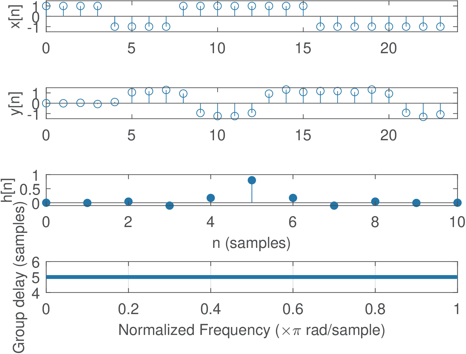
Figure 3.84: Linear phase FIR channel obtained with h=fir1(10,0.8). The output signal was scaled to have the same power as the input.

For example, consider the linear phase channel obtained with h=fir1(10,0.8). Figure 3.84 depicts its impulse response, group delay and the output $y [n]$ for an input $x [n]$ representing symbols $+ 1, - 1, + 1, + 1, - 1, - 1$ with an oversampling of $L = 4$ samples per symbol and a shaping pulse with four samples equal to 1.

Figure 3.84 allows to observe that the input gets delayed by the group delay of h, which in this case is 5. Note that the input peak at x[0] corresponds to the output sample y[5]. This simple signal delay happens because because h in this example was chosen to be symmetric and have a linear phase, such that the group delay is 5 samples for all frequencies as indicated in Figure 3.84. In terms of seconds, a group delay of 5 samples corresponds to $5 T_{s} = 5 ∕ F_{s}$ , where $F_{s}$ is given in Hz. In this case, the first 5 samples of the output should be eliminated for aligning with $x [n]$ . For example, the commands y(1:5)=[], x(end-4:end)=[] could be used to align the corresponding vectors and keep them with the same number of samples.

However, in a more general scenario, the group delay varies with frequency, such as for the non-symmetric FIR filter illustrated in Figure 3.56.

Typically a channel attenuates the input signal and decreases its power. When the channel is LTI, the output power $P_{y}$ is related to the input power $P_{x}$ as informed by Theorem 3 (page 1341).

When comparing the input $x [n]$ and output $y [n]$ waveforms, it is useful to know the ratio $g = P_{y} ∕ P_{x}$ and multiply $x [n]$ by $\sqrt{g}$ in order to compare signals with equivalent amplitude ranges. However, in practice, it is hard to determine $g$ and typically an adaptive automatic gain control (AGC) is employed.

Another example of compensating the delay and gain imposed by a channel is discussed in the sequel.

If useful, one can mimic a perfect automatic gain control (AGC) and force the output to have the same power as the input with the following commands Px=mean(x.^2), Py=mean(y.^2), y = sqrt(Px/Py)*y.

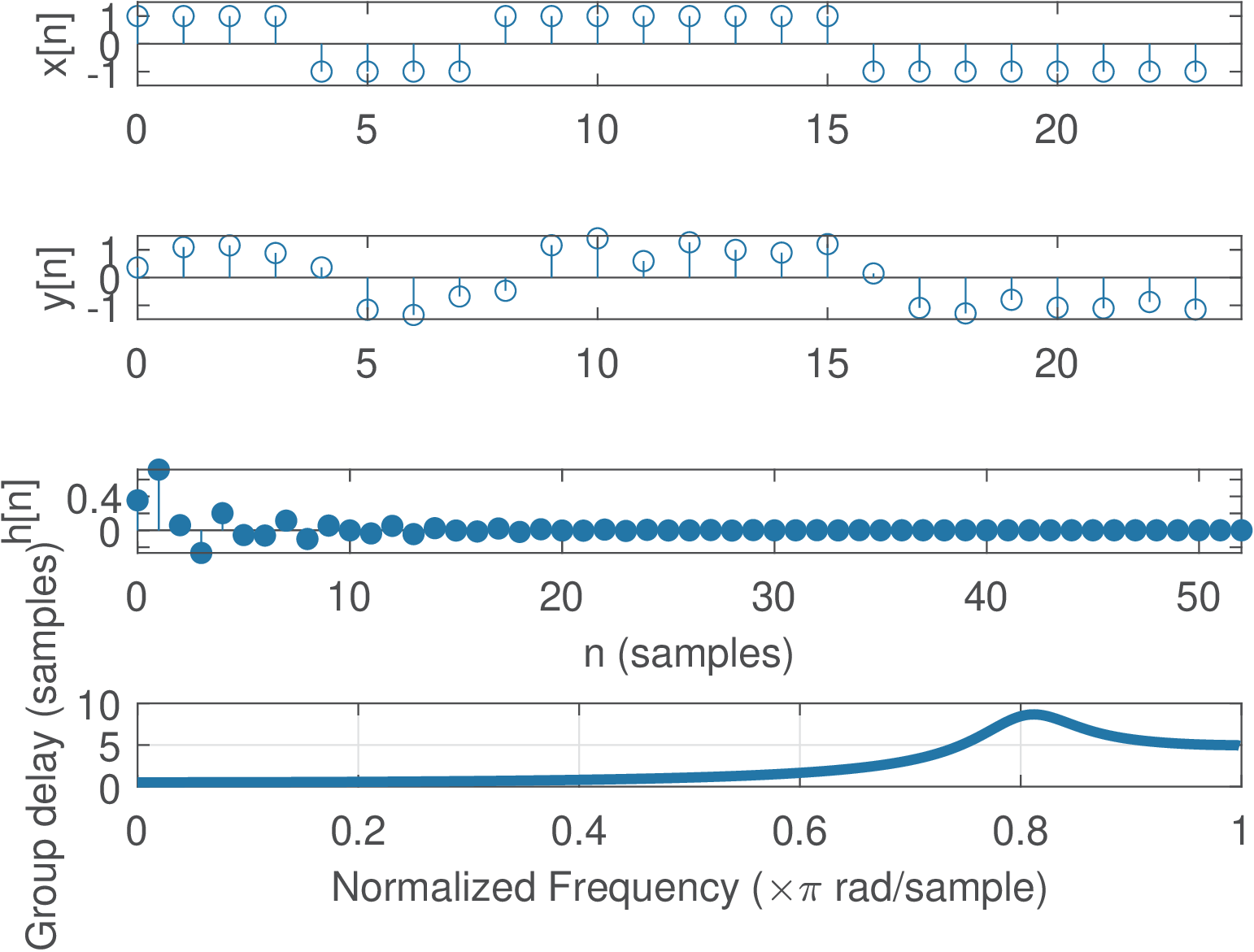
Figure 3.85: IIR channel obtained with [B,A]=butter(5,0.8). The output signal was scaled to have the same power as the input.

Similar to the procedure for generating Figure 3.84, an IIR filter was simulated to obtain Figure 3.85. In this case the group delay is less than 1 for frequencies $Ω < 0.47 π$ and the peak of $h [n]$ is for $n = 1$ . Observing the graphs of $x [n]$ and $y [n]$ , a good alignment would be obtained by shifting $y [n]$ one sample to the left, i. e., $y [n + 1]$ if manipulating algebraically or y(1)=[] if using Matlab/Octave. $□$