3.16  Advanced: Minimum phase systems

A LTI discrete-time system $H(z)$ is causal and stable only if all its poles are inside the unit circle, but these two requirements do not impose restrictions on the zeros. The zeros of a causal and stable $H(z)$ can be anywhere in the Z plane. In many cases, it is useful to impose that the zeros must also be inside the unit circle. For a continuous-time system $H(s)$, the equivalent requirement is to have all zeros inside the left-part of the S plane. A minimum-phase system has this property.

A LTI is minimum-phase if both the system $H$ itself and its inverse $1∕H$ are causal and stable. Assuming, discrete-time, because the poles of the inverse $1∕H(z)$ are the zeros of $H(z)$, only a system with all zeros inside the unit circle has a causal and stable inverse. Similarly, a continuous-time system $H(s)$ is minimum-phase only if all its zeros are at the left half of the S-plane.

A non-minimum-phase system $H_{\mathrm{\text{non}}}(z)$ can always be transformed into a minimum-phase $H_{\mathrm{\text{min}}}(z)$ that has the same magnitude, i. e., $|H_{\mathrm{\text{non}}}(z)|=|H_{\mathrm{\text{min}}}(z)|$. This is achieved by replacing the zeros of $H_{\mathrm{\text{non}}}(z)$ that are outside the unit circle by their conjugate reciprocals.³⁸ That is, replace all zeros $z_0$ with $|z_0|>1$ by $1∕z_0^{\ast }$. For example, if $z_0=2e^{\mathit{j\pi }∕2}$ is a zero of $H_{\mathrm{\text{non}}}(z)$, it should be replaced by $1∕z_0^{\ast }=0.5e^{\mathit{j\pi }∕2}$. The function ak_forceStableMinimumPhase.m implements this method and also decreases the magnitude of zeros on top of the unit circle.

1clf 
2B_roots = [2*exp(j*pi/4) 2*exp(-j*pi/4) ... %define roots 
3    0.7*exp(j*pi/8) 0.7*exp(-j*pi/8)]; 
4B=poly(B_roots) %construct B(z) of H(z)=B(z)/A(z) 
5A=poly([0.4 0.5 0.6 0.5j -0.5j 0.3j -0.3j]); %arbitrary 
6Bmin = ak_forceStableMinimumPhase(B) %move zeros inside 
7[H,w]=freqz(B,A); %frequency response for original H(z) 
8[Hmin,w]=freqz(Bmin,A); w=w/pi; %for minimum phase H(z) 
9subplot(211), plot(w,abs(H),w,abs(Hmin),'--'), axis tight 
10legend1 = legend('non-min','min-phase'), subplot(212)
  

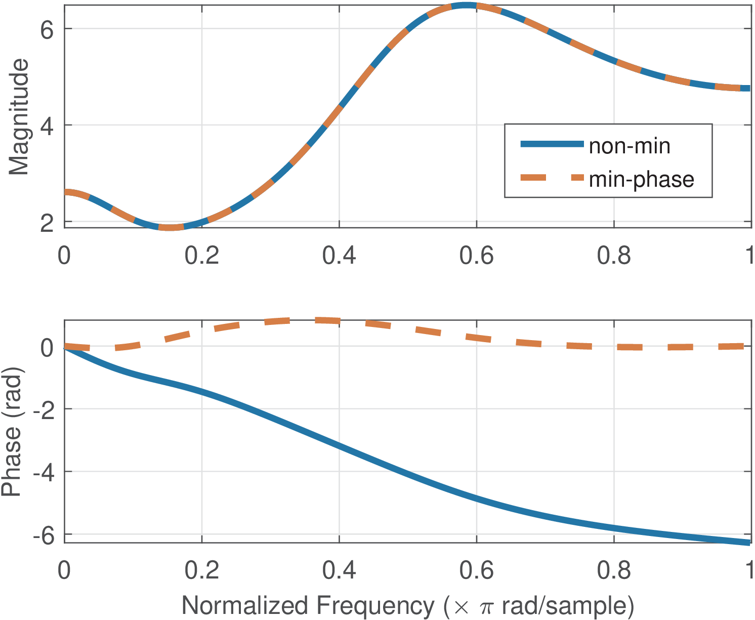
Figure 3.64 was obtained with Listing 3.39. Note that the magnitude is the same but the phase is distinct, with $H_{\mathrm{\text{min}}}(z)$ having smaller values.

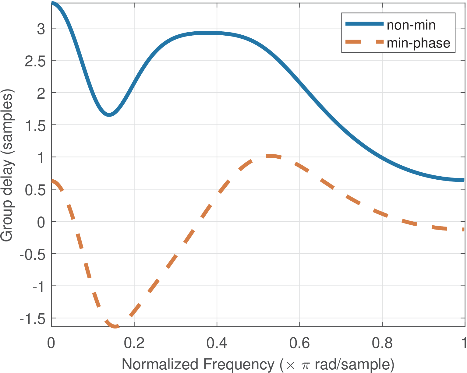
Minimum-phase systems have interesting properties. As the name indicates, among all systems with a given magnitude, the minimum-phase is the one with the phase closest to zero. Figure 3.64 illustrates this behavior, which can also be observed via the group delay, as in Figure 3.65.

Besides, the impulse response $h[n]$ of a minimum-phase system has its energy concentrated toward time $n=0$ more than any other causal signal having the same magnitude spectrum.