Advanced: First and Second-Order Analog Systems

3.6 Advanced: First and Second-Order Analog Systems

Because they are basic building blocks for higher-order filters, first and second-order continuous-time (also called analog) systems are discussed in the sequel.

3.6.1 First-order systems

If the coefficients are real, a first-order system $H (s) = 1 ∕ (s + a), a \in ℝ$ , (as the one whose frequency response is depicted in Figure 3.8) is restricted to have a lowpass frequency response. This $H (s)$ has a pole at $s = - a$ and a zero at $s = \infty$ . Using $H (s) = a ∕ (s + a)$ leads to a unitary gain at DC. Placing a zero at $s = 0$ leads to $H (s) = s ∕ (s + a)$ , which has a highpass response.

A system $H (s) = 1 ∕ (s + a)$ with ROC given by $σ > - a$ has an inverse Laplace transform $h (t) = e^{- at} u (t)$ , which can be written as $h (t) = e^{- t ∕ τ} u (t)$ where $τ$ is the well-known time constant [ url3mit]. After an interval of one time constant, the impulse response has decayed to 36.8% of its initial value.

If the ROC of $H (s) = a ∕ (s + a)$ includes $s = jω$ , the frequency response in this case is $H (ω) = a ∕ (jω + a)$ . As illustrated by Eq. (3.34), the magnitude $| H (ω) | = a ∕ \sqrt{a^{2} + ω^{2}}$ at $ω = a$ is then $| H (a) | = 1 ∕ \sqrt{2}$ , which is the cutoff frequency $ω_{c} = a$ because it corresponds to a decrease of 3 dB in power.

3.6.2 Second-order systems

The system function $H (s)$ of a second-order system (SOS), also called a two-pole resonator, has a denominator that can be written as $s^{2} + 2 αs + ω_{n}^{2}$ . When there are two zeros at $\infty$ and the gain at DC is unitary ( $H (s) |_{s = 0} = 1$ ), the SOS is:

H (s) = \frac{ω_{n}^{2}}{s^{2} + 2 αs + ω_{n}^{2}},

(3.27)

where $ω_{n}$ is the natural frequency and $α$ the decay rate parameter, which is useful for defining the damping ratio $ζ = α ∕ ω_{n}$ . Hence, Eq. (3.27) can be rewritten as:

H (s) = \frac{ω_{n}^{2}}{s^{2} + 2 ζ ω_{n} s + ω_{n}^{2}} .

(3.28)

The values of $α$ , $ζ$ and $ω_{n}$ can be related to several characteristics of a SOS. For example, $α$ represents the rate of exponential decay of oscillations when the system input is a unit step $u (t)$ . And depending on $ζ$ , three categories of second-order systems are defined:

$ζ = 1$ : critically damped SOS, with a double real pole at $- ω_{n}$ ;
$ζ > 1$ : overdamped SOS, with real poles at $- ζ ω_{n} \pm ω_{0}$ ;
$0 \leq ζ < 1$ : underdamped SOS, with complex conjugate poles.

Note that these three categories depend only on the denominator of $H (s)$ .

The numerator of $H (s)$ represents another degree of freedom. Changing this numerator, leads to distinct SOS. An alternative to Eq. (3.27) (or, equivalently, Eq. (3.28)) is

H (s) = \frac{s}{s^{2} + 2 ζ ω_{n} s + ω_{n}^{2}},

(3.29)

which has a zero at the origin ( $H (s) |_{s = 0} = 0$ ). Yet, other two options of SOS can be defined as

H (s) = \frac{s^{2}}{s^{2} + 2 ζ ω_{n} s + ω_{n}^{2}}

(3.30)

and

H (s) = \frac{2 ζ ω_{n} s + ω_{n}^{2}}{s^{2} + 2 ζ ω_{n} s + ω_{n}^{2}} .

(3.31)

Table 3.2 summarizes these options for the numerator of a SOS.

Table 3.2: Some distinct options for the numerator of a SOS.


Characteristic	Numerator	Reference

Two-zeros at $\infty$ and unitary DC gain	$ω_{n}^{2}$	Eq. (3.28)

One zero at DC	$s$	Eq. (3.29)

Two zeros at DC	$s^{2}$	Eq. (3.30)

One finite zero at $- ω_{n} ∕ (2 ζ)$	$2 ζ ω_{n} s + ω_{n}^{2}$	Eq. (3.31)

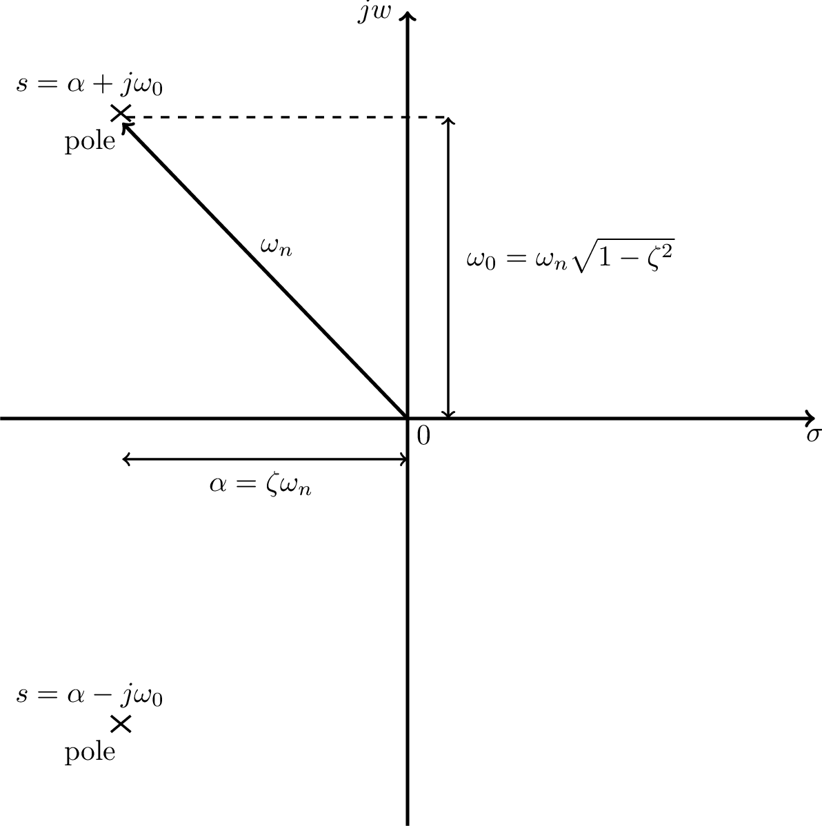
Using the quadratic formula to find the roots of a SOS, the poles are $s_{0} = - α \pm \sqrt{α^{2} - ω_{n}^{2}}$ , which can be rewritten as $s_{0} = - α \pm j \sqrt{ω_{n}^{2} - α^{2}}$ . Figure 3.19 summarizes these relations. Note that $ω_{n} = | s_{0} |$ and, unless $α = 0$ (poles on the $jω$ axis), the natural frequency $ω_{n}$ is different from the center frequency of the pole $ω_{0} = I mag {p} = \sqrt{ω_{n}^{2} - α^{2}} = ω_{n} \sqrt{1 - ζ^{2}}$ .

Figure 3.19: Relations between natural frequency $ω_{n}$ , pole center frequency $ω_{0}$ , decay rate $α$ and damping ratio $ζ$ for a pair of complex conjugate poles.

Note that for a first-order system $H (s) = a ∕ (s + a)$ with real-valued coefficient $a$ , the pole is real, its center frequency is $ω_{0} = 0$ , and the natural and cutoff frequencies $ω_{n} = ω_{c} = a$ coincide. For a second-order system, the expression for the cutoff frequency $ω_{c}$ is more elaborated. Considering Eq. (3.27), the cutoff is

ω_{c} = ω_{n} \sqrt{1 - 2 ζ^{2} + \sqrt{4 ζ^{4} - 4 ζ^{2} + 2}},

(3.32)

which can be found by using $| H (s) |_{s = j ω_{c}} = 1 ∕ \sqrt{2}$ . In this case, $ω_{c} = ω_{n}$ when $ζ = 1 ∕ \sqrt{2}$ .

Example 3.7. On the damping ratio of a SOS. Figure 3.20 illustrates the influence of the damping ratio using the values $ζ = 0.5, 0.707, 1$ and 2.

Figure 3.20: Magnitude of the frequency response for the SOS expressed by Eq. (3.28) and Eq. (3.31).

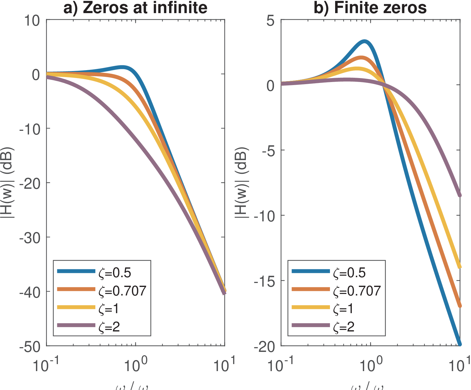
Figure 3.20 also compares Eq. (3.28) and Eq. (3.31), which are two of the options contrasted in Table 3.2. $□$

Figure 3.21 illustrates some key time-domain performance parameters for an underdamped system obtained when the input $x (t) = u (t)$ is a step function. The rise time $t_{r}$ is the interval for the step response to rise from 10 to 90% of its final value. The settling time $t_{s}$ is the interval to have the output within a given range, which is 5% in Figure 3.21. The overshoot is the peak amplitude and occurs at the peak time $t_{p}$ .

Figure 3.21: Time-domain performance parameters for an underdamped system based on its step response.

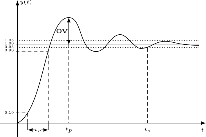
Table 3.3 summarizes some parameters for the system $H (s)$ described by Eq. (3.28), which can be found⁸ from the inverse Laplace transform of $Y (s) = H (s) ∕ s$ given that $X (s) = 1 ∕ s$ is the transform of $u (t)$ . The tolerance $𝜖$ is used to obtain $t_{s}$ and a typical value is $𝜖 = 0.05$ .

Table 3.3: Parameters of a second-order system as described by Eq. (3.28).


Performance parameter	Expression	For $ζ = \sqrt{2} ∕ 2 \approx 0.707$

Peak time	$t_{p} = π ∕ ω_{0} = π ∕ (ω_{n} \sqrt{1 - ζ^{2}})$	$t_{p} = 4.4 ∕ ω_{n}$

Rise time	$t_{r} \approx (2.23 ζ^{2} - 0.078 ζ + 1.12) ∕ ω_{0}$	$t_{r} = 3 ∕ ω_{n}$

Settling time	$t_{s} = - ln (𝜖 \sqrt{1 - ζ^{2}}) ∕ (ζ ω_{n})$	$t_{s} = 4.7 ∕ ω_{n}$

Overshoot	$ov = e^{- (ζπ) ∕ \sqrt{1 - ζ^{2}}}$	ov=4.32%

3-dB bandwidth $ω_{c}$ (rad/s)	$ω_{c} = ω_{n} \sqrt{1 - 2 ζ^{2} + \sqrt{2 - 4 ζ^{2} + 4 ζ^{4}}}$	$ω_{c} = ω_{n}$

Table 3.3 indicates that, for an underdamped system, the rise time when $ζ = \sqrt{2} ∕ 2$ is $t_{r} = 3 ∕ ω_{n}$ . As expected, all three time parameters are inversely proportional to the natural frequency $ω_{n}$ .

Listing 3.8 indicates the commands to calculate the parameters, emphasizing the factors that depend on $ζ$ (zeta) only.

Listing 3.8: MatlabOctaveCodeSnippets/snip_systems_sos_parameters.m. [ Python version]

1zeta=0.5 %damping ratio, e.g. sqrt(2)/2 = 0.707; 
2wn=2 %natural frequency in rad/s 
3epsilon=0.05 %tolerance for the settling time (5% in this case) 
4tp_factor=pi/sqrt(1-zeta^2) %depends on zeta only 
5tp=tp_factor/wn %peak time 
6tr_factor=(2.23*zeta^2 - 0.078*zeta + 1.12)/sqrt(1-zeta^2) %zeta only 
7tr=tr_factor/wn %rise time 
8ts_factor= -log(epsilon * sqrt(1-zeta^2))/(zeta) %zeta only 
9ts=ts_factor/wn %settling time 
10ov=exp(-(zeta*pi)/sqrt(1-zeta^2)) %overshoot (depends on zeta only) 
11bw_factor=sqrt(1-2*zeta^2 + sqrt(2 - 4*zeta^2 + 4*zeta^4)) %zeta only 
12wc=wn*bw_factor %cutoff frequency=3-dB bandwidth (in radians/second) 
13%% Check whether the cuttoff frequency wc corresponds to a -3 dB gain 
14s = 1j*wc %define s = j wc 
15Hs = (wn^2) / (s^2 + 2*zeta*wn*s + (wn^2)) % system function 
16gain_at_wc = 20*log10(abs(Hs))  %answer is -3.0103 dB

Matlab has the stepinfo function, which can be used to obtain most of the parameters in Table 3.3 as follows:

1zeta=0.5 %damping ratio, e.g. sqrt(2)/2 = 0.707; 
2wn=2 %natural frequency in rad/s 
3sys = tf([wn^2],[1 2*zeta*wn wn^2]); %define the transfer function 
4S=stepinfo(sys,'RiseTimeLimits',[0.1,0.9], ... 
5    'SettlingTimeThreshold',0.05) %get parameters with stepinfo 
6step(sys) %plot step response to check results if want

The system bandwidth will be discussed in the next section. Table 3.3 informs that, when $ζ = \sqrt{2} ∕ 2$ , the 3-dB bandwidth $ω_{c}$ in radians per second of the SOS given by Eq. (3.28) is simply its natural frequency $ω_{n}$ . In fact, as $ζ$ varies from 0.5 to 0.8, which are the values typically used, its $ω_{c}$ varies from $1.27 ω_{n}$ to $0.87 ω_{n}$ . This justifies using $ω_{n}$ as a rough approximation of bandwidth for Eq. (3.28).

⁸ These results can be found in textbooks of control systems or, e. g., [ url3con].