FIR Filter Design

3.14 FIR Filter Design

This section discusses filters that have impulse responses with finite duration.

3.14.1 A FIR filter does not have finite poles

Essentially, most FIR filters are non-recursive and have a transfer function that can be written as $H (z) = B (z)$ , i. e., the denominator is $A (z) = 1$ in Eq. (3.52). Given this denominator, all poles of FIR filters are located in $z = 0$ or $| z | = \infty$ (while IIR filters do not have this restriction). For example, $H (z) = 1 + z^{- 1} + z^{- 2}$ has a pole of order (or multiplicity) 2 at $z = 0$ . You can check that with zplane([1 1 1],1) on Matlab/Octave³⁴ or note it by rewriting as $H (z) = (z^{2} + z + 1) ∕ z^{2}$ . Another example is the noncausal system $H (z) = z^{2} + z + 1$ , which has a pole of multiplicity 2 at infinity.³⁵

3.14.2 The coefficients of a FIR coincide with its impulse response

An interesting property of FIR filters is that the coefficients of $H (z) = B (z)$ (also called “taps”) are exactly the non-zero values of the filter’s impulse response $h [n]$ . For example, using the inverse Z-transform on $H (z) = 3 + 4 z^{- 1} + 5 z^{- 2}$ , one obtains $h [n] = Z^{- 1} {H (z)} = 3 δ [n] + 4 δ [n - 1] + 5 δ [n - 2]$ .

This property sometimes leads to confusing commands. For instance, the arguments Bz and Az to method freqz(Bz,Az) are polynomials in Z transform domain. But for FIR filters, it is possible to substitute Bz by the impulse response hn as follows:

1hn=[2, 1, 3]; % define some arbitrary FIR impulse response 
2freqz(hn, 1); % find the DTFT corresponding to H(z)=B(z)/A(z)

Note in this code that $A (z) = 1$ for an FIR filter.

3.14.3 Algorithms for FIR filter design

Figure 3.47: Mask for a differentiator filter specified with the syntax for arbitrary filter magnitudes.

There are several algorithms for both FIR and IIR. Instead of using pre-defined functions such as Butterworth’s, a FIR design is typically done with alternative methods, which seek to optimize a given criterion. The most common algorithm is the least-squares, which is implemented in Matlab/Octave via firls. Another algorithm is Parks-McClellan, implemented in Matlab’s firpm, but not available in Octave 3.2.3.

These and other optimization-based algorithms are executed according to a syntax that allows specifying an arbitrary function, not restricted to be lowpass, highpass, etc. Figure 3.47 illustrates the specification of a desired magnitude response of a differentiator, which has a gain in passband that is proportional to frequency. An arbitrary function will be specified in $N_{B}$ bands of interest. For each band $b$ , four parameters are necessary: the start $f_{b}^{s}$ and end $f_{b}^{e}$ frequencies, the desired function values (the magnitude in this context) $A_{b}^{s}$ and $A_{b}^{e}$ at the start and end frequencies. An optional parameter is the weight of each band (e. g., W1 and W2 in Figure 3.47). The larger the weight, the higher the importance given to that band in the design process.

In Matlab/Octave, the function fir2 implements another algorithm for designing a FIR with arbitrary frequency response magnitude, using a different syntax. Instead of working with bands, fir2 allows the specification of the desired magnitude at frequencies of interest.

An example of using least-squares for FIR design with firls is discussed in the sequel.

3.14.4 FIR design via least-squares

The least-squares method tries to minimize the total squared error between the desired function and the obtained approximation over the specified band. It is possible to give a different weight to each band. The larger the weight, the smaller the error in that band. A vector W with weights is an optional input parameter of firls.

For example, an ideal lowpass with cutoff $Ω = π ∕ 2$ rad can be specified with $N_{B} = 2$ bands. The (normalized) frequencies could be $f_{1}^{s} = 0, f_{1}^{e} = 0.5, f_{2}^{s} = 0.5, f_{2}^{e} = 1$ and the amplitudes $A_{1}^{s} = 1, A_{1}^{e} = 1, A_{2}^{s} = 0, A_{2}^{e} = 0$ . These values are organized in vectors F=[0 0.5 0.5 1] and A=[1 1 0 0] and a $M = 100$ -order FIR can be obtained with B=firls(100,F,A). Note that A and F have the same length, which must be $2 N_{B}$ (even number), and W must have length equal to $N_{B}$ if specified. The default is to weight all bands equally, which corresponds to W with all elements equal to 1.

Figure 3.48: Frequency response of filters obtained with firls. In (a), the first passband had a larger weight than the second, while in (b) it was the opposite.

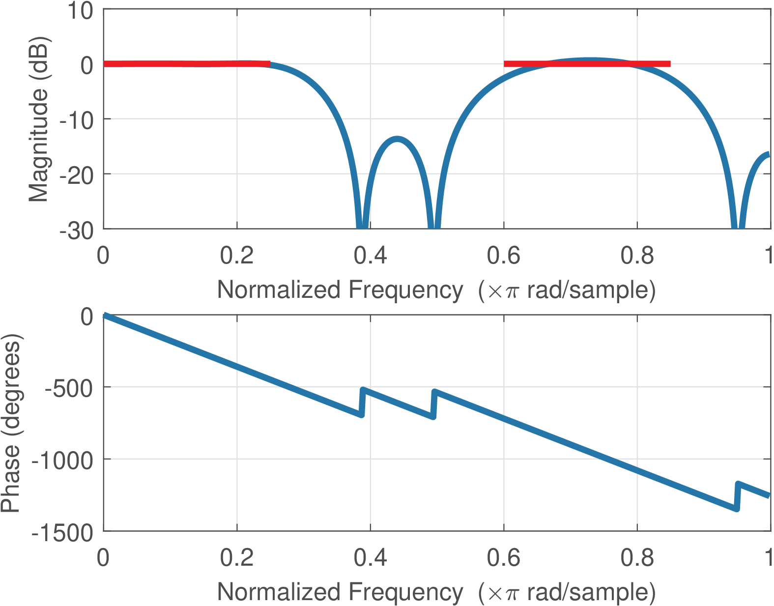
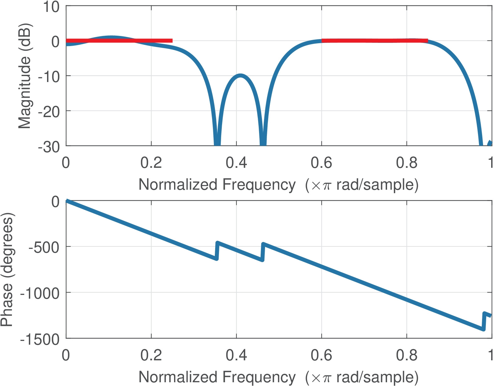
Figure 3.48 compares the frequency responses of two filters obtained with firls. Figure 3.48(a) was obtained with Listing 3.27.

Listing 3.27: MatlabOctaveCodeSnippets/snip_systems_firls.m. [ Python version]

1f=[0 0.25 0.3 0.55 0.6 0.85 0.9 1]; %frequencies 
2A=[1 1 0 0 1 1 0 0]; %amplitudes 
3M=20; %filter order 
4W=[1000 1 1 1]; %weights, first passband is prioritized 
5B=firls(M,f,A,W); 
6freqz(B);

The horizontal lines were superimposed to indicate the bands in which the gain should be 0 dB. Figure 3.48(b) was obtained with the same commands, but changing W to W=[1 1 1000 1]. Note that the impact of W is visible with the band that is not prioritized having larger deviations.

3.14.5 FIR design via windowing

The windowing method for FIR design is implemented in fir1. In terms of computational cost, the method is very simple: the FIR impulse response $h [n]$ is obtained by multiplying the impulse response of an ideal filter (which has an infinite duration) by a finite-length sequence $w [n]$ called window with $M + 1$ non-zero samples. Recall that the coefficients $B (z)$ of a FIR coincide with its $h [n]$ . For the case of an ideal lowpass filter, the impulse response is given by

h_{LP} [n] = \frac{sin (Ω_{c} n)}{πn},

(3.86)

which is the inverse DTFT of a “rectangular pulse” in frequency-domain.

The impulse response for the ideal highpass filter can be obtained by noting that $H_{HP} (e^{j Ω}) = 1 - H_{HP} (e^{j Ω})$ and converting this to time-domain leads to

h_{HP} [n] = δ [n] - h_{LP} [n] .

(3.87)

The steps to obtain a FIR filter $h_{w} [n]$ of order $M$ (assumed to be an even number here) via the windowing method are:

f 1.

Obtain the impulse response for the corresponding ideal filter:

h [n]

has an infinite duration but the next steps will require only

M + 1

of its coefficients.

f 2.

Choose a window: Pick a window

w [n]

with

M + 1

non-zero coefficients in the range

[- M ∕ 2, M ∕ 2]

f 3.

Get a filter with finite order

M

(i. e.,

M + 1

coefficients): Multiply the chosen window

w [n]

by the ideal filter impulse response

h [n]

to get a temporary

h_{w}^{t} [n] = h [n] w [n] .

(3.88)

f 4.

Make the filter causal: Delay

h_{w}^{t} [n]

such that the first

h_{w} [n]

coefficient is at

n = 0

h_{w} [n] = h_{w}^{t} [n - M ∕ 2] .

(3.89)

The DTFT of $h [n]$ , $w [n]$ , $h_{w}^{t} [n]$ and $h_{w} [n]$ are $H (e^{j Ω})$ , $W (e^{j Ω})$ , $H_{w}^{t} (e^{j Ω})$ and $H_{w} (e^{j Ω})$ , respectively. Figure 3.49 illustrates the effect of multiplying a signal ( $h [n]$ in this case) by a finite-duration window. This is a very useful approach for modeling the process of truncating an infinite-duration signal for further processing. This model allows to calculate, for instance, the spectrum of the finite-duration signal based on the convolution between the original and the window spectra. This is useful not only in FIR design, but many other situations such as segmenting a signal into frames.

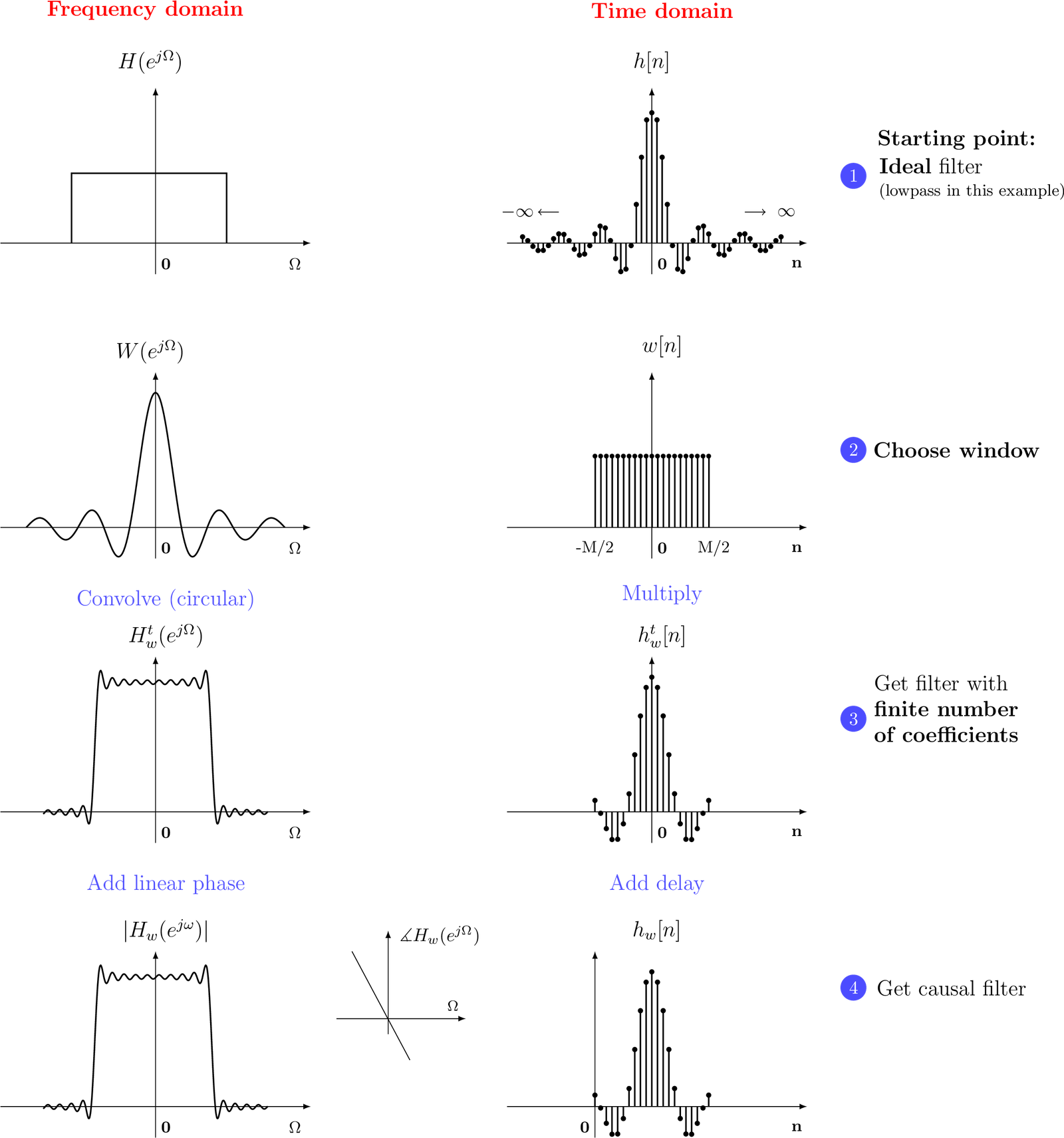
Figure 3.49: FIR design described in both time and frequency domains.

In windows-based FIR design, the filter frequency response $H_{w} (e^{j Ω})$ is the result of the (circular) convolution between $H (e^{j Ω})$ and $W (e^{j Ω})$ , as indicated in Figure 3.49. The ripples (ringing) observed in $H_{w} (e^{j Ω})$ are located at the transitions of $H (e^{j Ω})$ and indicate that the main lobe of $W (e^{j Ω})$ dictates the transition band and the amplitude of $W (e^{j Ω})$ sidelobes determine the attenuation at the stopband.

The properties of the filter are completely dependent on the adopted window type. The most common windows are named after their inventors: Hamming, Blackman, Kaiser and Hann (also called the hanning window). Among these four, the Kaiser is the only one with an extra degree of freedom provided by a parameter $β$ . The other three are completely specified by the order $M$ .

The rectangular window is useful to better understand the windowing process. The rectangular is 1 for $M + 1$ samples and 0 otherwise. For example, a $4$ -th order lowpass filter with $Ω_{c} = π ∕ 3$ can be designed with a rectangular windows according to Listing 3.28.

Listing 3.28: MatlabOctaveCodeSnippets/snip_systems_rectangular_window.m

1%% Low pass FIR design via windowing 
2N=2; %the FIR order is M=2N in this case 
3n=-N:N; %time indices 
4wc = pi/3 %specified cutoff frequency 
5h_ideal = sin(wc * n) ./ (pi * n) %ideal filter response 
6h_ideal(N+1)=wc/pi %correct undetermined value 0/0 at n=0 
7%% "Manually" design FIR with rectangular window 
8% a rectangular window has values 1, no need to multiply 
9hn = h_ideal/sum(h_ideal) %normalize to have gain 1 at DC 
10%% "Automatically" design FIR using windowing via fir1 
11B=fir1(2*N,wc/pi,rectwin(2*N+1)) %alternatively, use fir1 
12max(abs(hn-B)) %compare hn with B obtained with fir1 
13%% "Manually" design (another) FIR with Hamming window 
14window_hamming = transpose(hamming(2*N+1)); %window 
15hn = h_ideal .* window_hamming; %multiply in time-domain 
16hn = hn/sum(hn) %normalize filter to have gain 1 at DC 
17%% "Automatically" design FIR using windowing via fir1 
18B=fir1(2*N,wc/pi,hamming(2*N+1)) %alternatively, use fir1 
19max(abs(hn-B)) %compare hn with B obtained with fir1

There is support in Matlab/Octave for obtaining windows other than the rectangular. For example, the command w=window(@hamming,10) obtains a Hamming window with 10 non-zero samples, which can be used to obtain a FIR of order $M = 9$ with cutoff frequency $Ω = π ∕ 2$ rad via the command B=fir1(9,0.5,w).

The adopted window determines the frequency response of the associated FIR designed via windowing. Section 4.3 discusses the characteristics of windows in more details.

One tricky feature of fir1 is that it generates filters with cutoff frequency $Ω_{c}$ that corresponds to a gain of $- 6$ dB (0.5 in linear scale). In contrast, the cutoff frequency of a filter obtained with butter and other IIR filter design functions corresponds to a gain of $- 3$ dB ( $1 ∕ \sqrt{2}$ in linear scale). Another aspect is that, if the order $M$ is too small when using fir1, the gain at $Ω_{c}$ may not reach $- 6$ dB. This also happens with other filter design procedures.

3.14.6 Two important characteristics: FIRs are always stable and can have linear phase

Because practical FIR filters have all $M + 1$ coefficients with finite values, Eq. (A.123) indicates that all FIR filters are BIBO stable. Besides, FIR filters can easily have linear phase, which is a desirable property in many applications (such as telecommunications, as will be discussed in Application 3.10). It can be proved that the linear phase is achieved if and only if there is symmetry in $h [n]$ about some value $n_{s}$ . For example, a FIR $H (z) = 1.5 - 2 z^{- 1} + 5 z^{- 2} - 2 z^{- 3} + 1.5 z^{- 4}$ of order $M = 4$ has 5 non-zero samples in $h [n]$ and exhibit symmetry about $n_{s} = 2$ , which corresponds to $h [2] = 5$ , such that $h [n] = h [4 - n]$ . The phase is linear over frequency because, for the given example:

\begin{align} H (e^{j Ω}) & = F {h [n]} & (3.90) \\ = F {1.5 δ [n] - 2 δ [n - 1] + 5 δ [n - 2] - 2 δ [n - 3] \\ + 1.5 δ [n - 4]} & (3.91) \\ = 1.5 - 2 e^{- j Ω} + 5 e^{- j 2 Ω} - 2 e^{- j 3 Ω} + 1.5 e^{- j 4 Ω} & (3.92) \\ = e^{- j 2 Ω} (1.5 e^{j 2 Ω} - 2 e^{j Ω} + 5 - 2 e^{- j Ω} + 1.5 e^{- j 2 Ω}) & (3.93) \\ = e^{- j 2 Ω} [1.5 (e^{j 2 Ω} + e^{- j 2 Ω}) - 2 (e^{j Ω} + e^{- j Ω}) + 5] & (3.94) \\ = e^{- j 2 Ω} [3 cos (2 Ω) - 4 cos (Ω) + 5] & (3.95) \\ = e^{- j 2 Ω} A (Ω), & (3.96) \end{align}

where $A (Ω) = 3 cos (2 Ω) - 2 cos (Ω) + 5$ is a real function that provides the magnitude $| H (e^{j Ω}) |$ , such that the phase $e^{- j 2 Ω}$ of $H (e^{j Ω})$ is linear $- 2 Ω$ , given by the factor .

As Eq. (3.96) indicates, a symmetric FIR can always be decomposed as

H (e^{j Ω}) = e^{- j Ω τ_{g}} A (Ω),

where $A (Ω)$ is a real function and $τ_{g}$ is the group delay, to be further discussed along with Eq. (3.45).

3.14.7 Examples of linear and non-linear phase filters

When the system has linear phase it is relatively easy to calculate its group delay because it coincides with the slope of a straight line. Listing 3.29 uses the FIR from Eq. (3.96) to show an example of calculating the slope from two points k1 and k2, comparing it with the result of the grpdelay function:

Listing 3.29: Group delay estimation for linar phase system

1h=[1.5 -2 5 -2 1.5]; %coefficients of symmetric FIR 
2N=8; %number of FFT points 
3Fs=44100; %sampling frequency (Hz) 
4H=fft(h,N); %calculate FFT of N points 
5f=Fs/N*(0:N/2); %create abscissa in Hz, where Fs/N is the bin width 
6p = unwrap(angle(H(1:N/2+1))); %calculate the phase in rad 
7plot(f,p), xlabel('f (Hz)'), ylabel('Phase (rad)'), pause 
8k1=2; k2=4; %choose two points of the line 
9%Calculate derivative as the slope. Convert from Hz to rad/s first: 
10groupDelay = -atan2(p(k2)-p(k1),2*pi*(f(k2)-f(k1))) %in seconds 
11groupDelayInSamples=round(2*groupDelay*Fs)/2; %quantize with step=0.5 
12grpdelay(h,1,f(1:N/2+1),Fs); %find delay for positive frequencies

Line 11 used round to avoid numerical errors. The trick of multiplying by 2 and after rounding divide by 2 allows to take into account that a symmetric FIR, unless the estimation was troubled due to the existence of zeros on the unit circle, has group delay that can be represented with a quantizer of step $Δ = 0.5$ sample.

Figure 3.50 and Figure 3.51 were obtained by executing Listing 3.30 for the filters [0.3 -0.4 0.5 0.8 0.5 -0.4 0.3] and [0.3 -0.4 0.5 0.8 -0.2 0.1 0.5], respectively.

Listing 3.30: Code for plotting the group delay and phase.

1function ak_plotGroupDelay(B,A) 
2% function ak_plotGroupDelay(B,A) 
3%Plots both the group delay and phase using plotyy 
4gd = grpdelay(B,A,128); %estimate the group delay 
5gd(1) = []; %avoid NaN at first sample 
6[H,w] = freqz(B,A,128); %obtain DTFT at 128 points 
7H(1) = []; w(1) = []; %keep the same size as gd vector 
8phase = unwrap(angle(H)); %unwrap the phase for better visualization 
9ax=plotyy(w,gd,w,phase); %use two distinct y axes 
10ylabel(ax(1),'Group Delay (samples)'); ylabel(ax(2),'Phase (rad)'); 
11xlabel('Frequency \Omega (rad)'); grid;

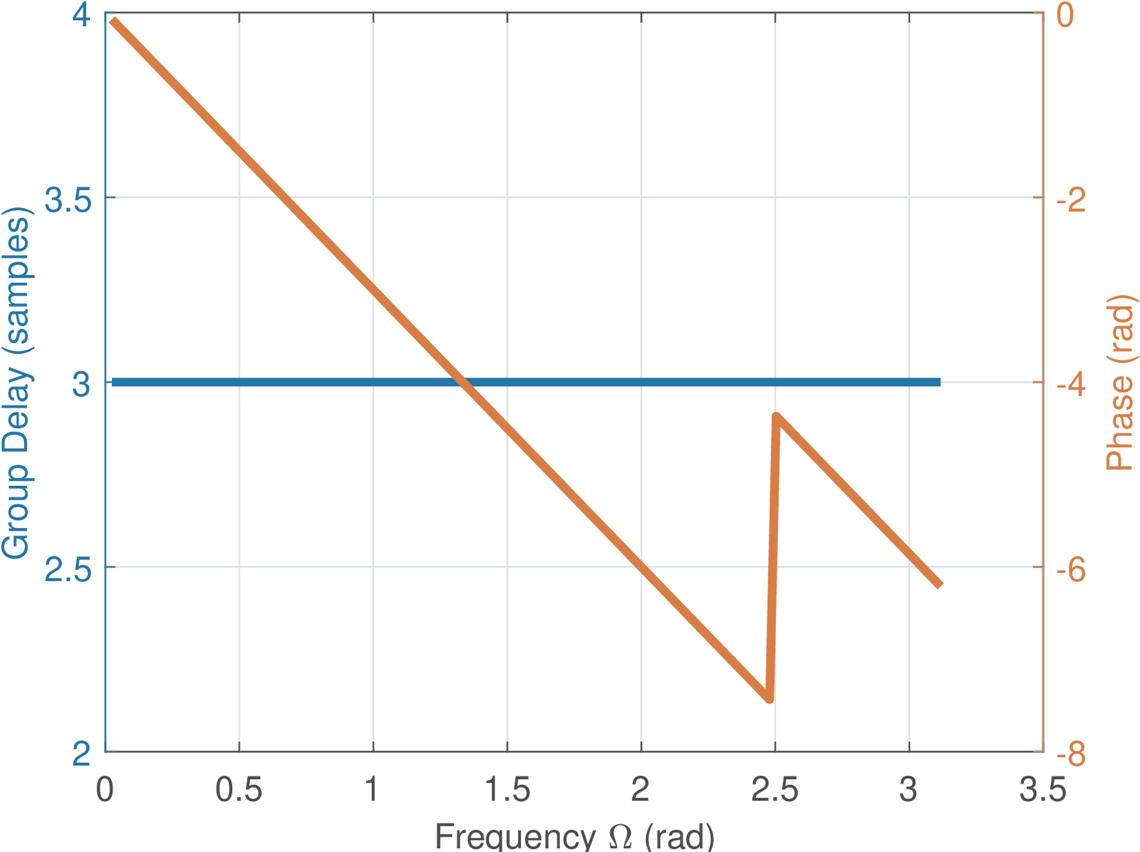
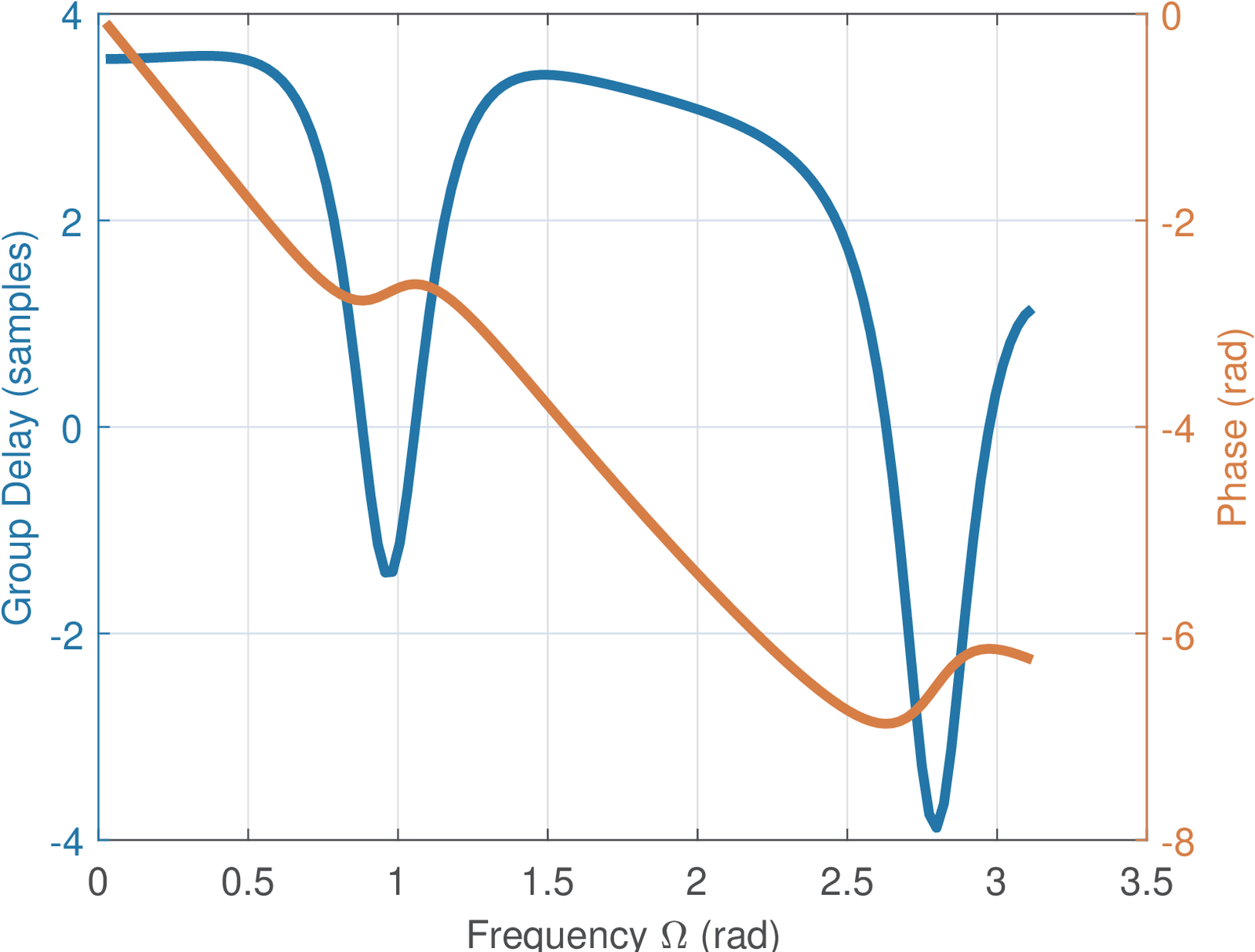
Figure 3.50: Group delay and phase for a channel represented by a symmetric FIR with linear phase and constant group delay of 3 samples.

Figure 3.51: Group delay and phase for a channel represented by a non-symmetric FIR h=[0.3 -0.4 0.5 0.8 -0.2 0.1 0.5] with non-linear phase.

The filter of Figure 3.50 has a linear phase while the one in Figure 3.51 does not. It can be seen from Figure 3.51 that even causal systems can have a negative group delay for some frequencies.

3.14.8 Zeros close to the unit circle may impact the phase linearity

An often overlooked fact is that if $A (Ω)$ approaches zero, the phase graph is not guaranteed to be visualized as a linear function of $Ω$ . For example, the first filter (from Eq. (3.96)) in the script below shows a linear phase via the freqz function, but the second does not due to a zero at approximately $e^{\pm j 1.994}$ :

1h1=[1.5 -2 5 -2 1.5]; freqz(h1); pause %has linear phase 
2h2=[-0.7 6 4 6 -0.7]; freqz(h2); %does not have linear phase 
3abs(roots(h2)), angle(roots(h2));%h2 has zeros on unit circle!

The function grpdelay properly treats the zeros on the unit circle and indicates $τ_{g} = 2$ samples for both h1 and h2 filters. Because conventional filters such as lowpass and bandpass do not have zeros at the passband, the symmetry of their coefficients guarantees linear phase within the band of interest and the discussed behavior often manifest itself only in the stopband.

Another way of interpreting the problem caused by zeros on the unit circle is to note that they lead to a zero magnitude. If the magnitude of a complex number is zero or close enough to zero, its phase will not be important.

3.14.9 Four types of symmetric FIR filters

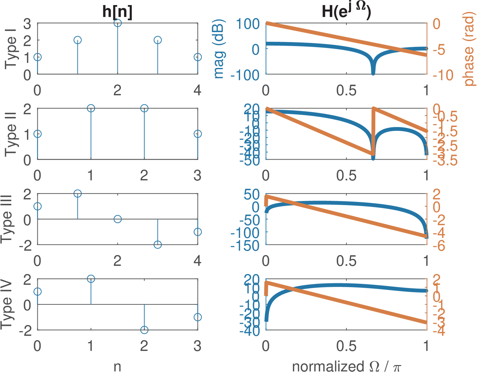
Depending on the symmetry, there are four types of linear-phase FIR filters. The filter of Eq. (3.96) is classified as a linear-phase FIR of type I. In general, a type I has an order $M$ that is even (the length of $h [n]$ is odd) and is symmetric $h [n] = h [M - n]$ . Table 3.9 summarizes all types.

Table 3.9: Types of linear-phase FIR filters. It is assumed that the filters are causal with the first non-zero sample at

n = 0

. Type III filters have

h [M ∕ 2] = 0

Type	Symmetry	Order ( $M$ )	$H (e^{j Ω}) \|_{Ω = 0}$ (DC)	$H (e^{j Ω}) \|_{Ω = π}$ (Nyquist)
I	Symmetric: $h [n] = h [M - n]$	even	any value	any value
II	Symmetric: $h [n] = h [M - n]$	odd	any value	0
III	Anti-symmetric: $h [n] = - h [M - n]$	even	0	0
IV	Anti-symmetric: $h [n] = - h [M - n]$	odd	0	any value

Recall that, because $H (e^{j Ω}) |_{Ω = 0} = H (z) |_{z = 1}$ , the behavior of a FIR filter at DC can be obtained with

H (z) |_{z = 1} = \sum_{k = 0}^{M} b_{k} = \sum_{n = 0}^{M} h [n] .

Hence, the anti-symmetric filters in Table 3.9 are restricted to have a zero at DC. Similarly, at the Nyquist frequency $Ω = π$ rad, $H (e^{j Ω}) |_{Ω = π} = H (z) |_{z = - 1}$ , and for a type III FIR with order $M$ even:

\begin{array}{l} H (z) |_{z = - 1} & = \sum_{k = 0}^{M} b_{k} = \sum_{k = 0}^{M ∕ 2} [b_{2 k} {(- 1)}^{2 k} + b_{2 k + 1} {(- 1)}^{2 k + 1}] \\ = \sum_{n = 0}^{M ∕ 2} (h [2 n] - h [2 n + 1]) = h [M ∕ 2] = 0, \end{array}

where the first parcels in the summations correspond to even ( $2 k$ or $2 n$ ) and the second parcels to odd coefficients. This kind of relation is better visualized via examples as in Listing 3.31.

Listing 3.31: MatlabOctaveCodeSnippets/snip_systems_FIR_types.m

1hI=[1 2 3 2 1] %Type I FIR 
2hII=[1 2 2 1]  %Type II FIR 
3hIII=[1 2 0 -2 -1] %Type III FIR 
4hIV=[1 2 -2 -1] %Type IV FIR 
5disp(['I: DC=' num2str(polyval(hI,1)) ... 
6    ' Nyquist=' num2str(polyval(hI,-1))]) 
7disp(['II: DC=' num2str(polyval(hII,1)) ... 
8    ' Nyquist=' num2str(polyval(hII,-1))]) 
9disp(['III: DC=' num2str(polyval(hIII,1)) ... 
10    ' Nyquist=' num2str(polyval(hIII,-1))]) 
11disp(['IV: DC=' num2str(polyval(hIV,1)) ... 
12    ' Nyquist=' num2str(polyval(hIV,-1))])

Running Listing 3.31 outputs

I: DC=9 Nyquist=1
II: DC=6 Nyquist=0
III: DC=0 Nyquist=0
IV: DC=0 Nyquist=2

as expected from Table 3.9. Because the gain at DC is zero, linear-phase FIR filters of type III and IV are useful to operate as differentiator filters, for example.

Figure 3.52 shows the impulse and frequency responses for the four types of symmetric FIR filters exemplified in Listing 3.31. Note that the type II FIR in this case (hII=[1 2 2 1]) has three zeros on the unit circle (use abs(roots(hII))) and its phase has a discontinuity in spite of a constant group delay (use grpdelay(hII)), as warned in Section 3.14.8.

Figure 3.52: Impulse and frequency responses for the four types of symmetric FIR filters exemplified in Listing 3.31.

³⁴ Note that Matlab shows the pole multiplicity in zplane while Octave version 3.2.3 does not.

³⁵ See [ url3poi] for a brief discussion about poles at infinity.