Bilinear Transformation: Definition and Properties

3.12 Bilinear Transformation: Definition and Properties

The most popular approach to designing conventional lowpass, highpass, bandpass and bandstop IIR filters is the bilinear transformation because it is capable of preserving in $H (z)$ , most of the good features of the original $H (s)$ . In this method, the discrete-time system function is obtained by:

H (z) = H (s) |_{s = \frac{2}{T_{s}} \frac{z - 1}{z + 1}} = H (s) |_{s = 2 F_{s} \frac{z - 1}{z + 1}} .

(3.64)

The bilinear is not a “transform” that relies on basis functions such as Fourier and Z. Instead, it is a simple tranformation from $H (s)$ in continuous-time to $H (z)$ in discrete-time.²³ The following examples illustrate the bilinear transformation.

Example 3.21. Examples of bilinear transformations. Assuming $F_{s} = 1000$ Hz, the bilinear transformation of $H (s) = \frac{1}{s + 2}$ (used in Figure 3.8) is

H (z) = \frac{1}{2 F_{s} \frac{(z - 1)}{z + 1} + 2} = \frac{1}{2002} (\frac{z + 1}{z - \frac{1998}{2002}}) = 4.995 \times 1 0^{- 4} (\frac{z + 1}{z - 0.998}) .

(3.65)

This operation can be very tedious when the order of $H (s)$ is high. But Python (scipy.signal.bilinear) and Matlab/Octave have the handy bilinear function. The result in Eq. (3.65) could be obtained with [HzNum,HzDen]=bilinear(1,[1 2],1000) in Matlab and [HzNum,HzDen]=bilinear(1,[1 2],1/1000) in Octave. In Python, the commands are:

1import scipy.signal 
2Bs=1; # numerator B(s) in continuous-time 
3As=[1, 2];  # denominator A(s) in continuous-time 
4Fs=1000 # sampling rate in Hz 
5[Bz, Az]=scipy.signal.bilinear(Bs, As, Fs) 
6print("Numerator B(z) =", Bz, " and Denominator A(z) =", Az)

Note that while Python’s and Matlab’s bilinear functions assume the sampling frequency $F_{s}$ as an input parameter, Octave adopts the sampling interval $T_{s} = 1 ∕ F_{s}$ . The first (Python’s and Matlab’s) syntax will be adopted here unless otherwise stated.

As an alternative to dealing with polynomials $B (s)$ and $A (s)$ , it is possible to use bilinear with the roots of these polynomials, by providing the poles and zeros of $H (s) = B (s) ∕ A (s)$ . In Matlab, the same $H (z)$ in Eq. (3.65) could be obtained using the poles and zeros of $H (s)$ , with: [HzZeros,HzPoles,gain]=bilinear([],-2,1,1000).

As a second example, consider the conversion of $H (s) = (s - 3) ∕ (s^{2} + 4 s + 5)$ (the poles are $- 2 \pm j$ and the zero is $3$ ) assuming $F_{s} = 10$ Hz:

H (z) = \frac{\frac{2}{T_{s}} \frac{z - 1}{z + 1} - 3}{{(\frac{2}{T_{s}} \frac{z - 1}{z + 1})}^{2} + 4 (\frac{2}{T_{s}} \frac{z - 1}{z + 1}) + 5} = \frac{0.035 - 0.012 z^{- 1} - 0.047 z^{- 2}}{1 - 1.629 z^{- 1} + 0.670 z^{- 2}}

which can be obtained in Matlab with the command [HzNum,HzDen]=bilinear([1 -3],[1 4 5],10).
An alternative call would be [HzZeros,HzPoles,gain]=bilinear(3,transpose([-2+j -2-j]),1,10) that leads to

H (z) = \frac{0.035 (z + 1) (z - 1.353)}{(z - 0.81 + j 0.082) (z - 0.81 - j 0.082)} .

(3.66)

But note that when using the function bilinear with poles and zeros in Matlab, one needs to use column instead of the row vectors used with transfer functions. $□$

Example 3.22. Bilinear transformation of second order $H (s)$ systems using symbolic math. Symbolic math can be used to conveniently perform algebraic manipulations, such as the bilinear transformation. In Matlab, the second order $H (s)$ given by Eq. (3.28) can be converted to a discrete-time version $H (z)$ using Listing 3.21.

Listing 3.21: MatlabOctaveCodeSnippets/snip_systems_sos_bilinear.m. [ Python version]

1%define s, z, natural frequency, damping ratio and sampling interval 
2syms s z wn zeta Ts %all as symbolic variables 
3Hs=wn^2/(s^2+2*zeta*wn*s+wn^2) %H(s). Use pretty(Hs) to see it 
4%Hs=(2*zeta*wn*s+wn^2)/(s^2+2*zeta*wn*s+wn^2) %Another H(s) 
5Hz=subs(Hs,s,(2/Ts)*((z-1)/(z+1))) %bilinear: s <- 2/Ts*(z-1)/(z+1) 
6Hz=simplify(Hz) %simplify the expression 
7pretty(Hz) %show it using an alternative view

The bilinear transformation of Eq. (3.28) is obtained as

H (z) = \frac{ω_{n}^{2} {T_{s}}^{2} {(z + 1)}^{2}}{(4 + 4 ζ ω_{n} T_{s} + {(ω_{n} T_{s})}^{2}) z^{2} + (2 {(ω_{n} T_{s})}^{2} - 8) z + 4 - 4 ζ ω_{n} T_{s} + {(ω_{n} T_{s})}^{2}},

(3.67)

which can be simplified using Eq. (1.36), i. e., substituting $ω_{n} T_{s} = Ω_{n}$ to obtain

H (z) = \frac{Ω_{n}^{2} {(z + 1)}^{2}}{(4 + 4 ζ Ω_{n} + Ω_{n}^{2}) z^{2} + (2 Ω_{n}^{2} - 8) z + 4 - 4 ζ Ω_{n} + Ω_{n}^{2}} .

(3.68)

Similarly, Listing 3.21 can be used to find the bilinear transformation of Eq. (3.31) as

H (z) = \frac{(4 ζ Ω_{n} + Ω_{n}^{2}) z^{2} + 2 Ω_{n}^{2} z + Ω_{n} (Ω_{n} - 4 ζ)}{(4 + 4 ζ Ω_{n} + Ω_{n}^{2}) z^{2} + (2 Ω_{n}^{2} - 8) z + 4 - 4 ζ Ω_{n} + Ω_{n}^{2}} .

(3.69)

Listing 3.22 can be used to verify Eq. (3.67) and Eq. (3.69)

Listing 3.22: MatlabOctaveCodeSnippets/snip_systems_check_sosbilinear.m. [ Python version]

1wn=2; %natural frequency in rad/s 
2zeta=0.5; %damping ratio 
3Fs=10*wn/(2*pi); %Fs chosen as 10 times the natural freq. in Hz 
4Wn=wn*(1/Fs); %convert angular freq. from continuous to discrete-time 
5if 1 %Hs=wn^2/(s^2+2*zeta*wn*s+wn^2) 
6    [Bz,Az]=bilinear(wn^2,[1 2*zeta*wn +wn^2],Fs) %to compare below 
7    Bz2=Wn^2*[1 2 1]; %expression from this textbook 
8    Az2=[4+4*zeta*Wn+Wn^2 2*Wn^2-8 4-4*zeta*Wn+Wn^2]; %from textbook 
9else %Hs=(2*zeta*wn*s+wn^2)/(s^2+2*zeta*wn*s+wn^2) %Another H(s) 
10    [Bz,Az]=bilinear([2*zeta*wn wn^2],[1 2*zeta*wn +wn^2],Fs)%compare 
11    Bz2=[4*zeta*Wn+Wn^2 2*Wn^2 Wn*(Wn-4*zeta)]; %from textbook 
12    Az2=[4+4*zeta*Wn+Wn^2 2*Wn^2-8 4-4*zeta*Wn+Wn^2]; %from textbook 
13end 
14Bz2=Bz2/Az2(1), Az2=Az2/Az2(1) %normalize as done by bilinear.m

Together, Listing 3.21 and Listing 3.22 indicate the power of combining symbolic math and numerical functions. $□$

Derivation of the bilinear transformation

There are several ways to explain and/or motivate the bilinear method. One of them is by modifying the matched Z-transform of Eq. (2.59), which relates z and s by $z = e^{s T_{s}}$ . Multiplying this relation by $e^{- s T_{s} ∕ 2} ∕ e^{- s T_{s} ∕ 2}$ and using the Taylor expansion $e^{x} = 1 + x + x^{2} ∕ 2 + \dots$ truncated to the first order $e^{x} \approx 1 + x$ , leads to²⁴

z \overset{def}{=} e^{s T_{s}} = \frac{e^{s T_{s} ∕ 2}}{e^{- s T_{s} ∕ 2}} \approx \frac{2 + s T_{s}}{2 - s T_{s}} .

(3.70)

Solving for $s$ , one obtains the bilinear transformation:

s \approx \frac{2}{T_{s}} [\frac{z - 1}{z + 1}]

(3.71)

and, therefore, the conversion is performed with Eq. (3.64).

The approximation $e^{x} \approx 1 + x$ requires $x$ to be close to 0, which in the bilinear transformation corresponds to having $s T_{s} \approx 0$ , i. e., having $T_{s}$ small enough (a high sampling frequency) for the values of $s$ of interest.

3.12.1 Bilinear mapping between s and z planes and vice-versa

Figure 3.33: Examples (a) and (b) of bilinear mappings from the unit circle in z to s plane. Mappings (c) and (d) of chosen points in s to z plane. Each example shows the points identified by numbers in their original and mapped planes.

Eq. (3.64) imposes a mapping between the s and z planes that depends only on $F_{s}$ . The code ak_map_s_into_z.m and ak_map_z_into_s.m allows to explore the mapping from s into z and vice-versa, respectively. The first mapping (from Eq. (3.64)) is

s = \frac{2}{T_{s}} \frac{z - 1}{z + 1}

(3.72)

and the mapping from s to z can be derived by isolating z:

z = \frac{2 + T_{s} s}{2 - T_{s} s} .

(3.73)

Example 3.23. Interpreting the mapping imposed by the bilinear transformation. According to Eq. (3.64), the bilinear transformation obtains the value of $H (z_{0})$ for a given $z_{0}$ , from the value of $H (s) |_{s = \frac{2}{T_{s}} \frac{z_{0} - 1}{z_{0} + 1}}$ . For instance, assuming $z_{0} = 3 + j 4$ and $T_{s} = 0.5$ seconds, then $H (z_{0}) = H (s) |_{s = 0.75 + j 0.25}$ . To avoid confusion and disambiguate $H (z)$ and $H (s)$ , it is useful to use a subindex and denote them $H_{z} (z)$ and $H_{s} (s)$ , respectively. The result of the previous example can now be conveniently written as $H_{z} (3 + j 4) = H_{s} (0.75 + j 0.25)$ . $□$

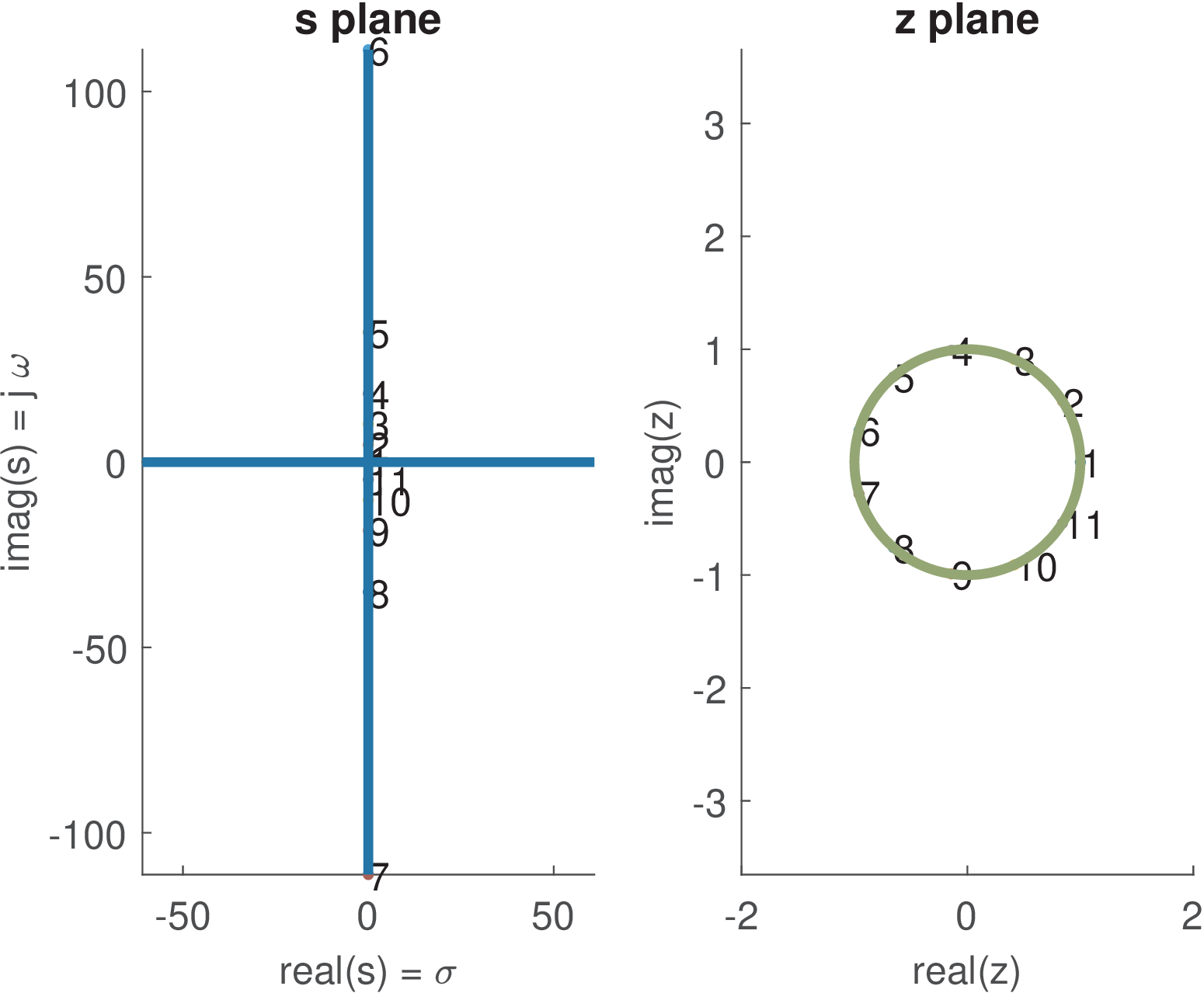
Figure 3.33 shows some examples of the mapping imposed by the bilinear transformation. Figure 3.33(a) illustrates how 11 points uniformly spaced in the unit circle of the plane z are mapped to s when assuming $F_{s} = 8$ Hz. Their corresponding positions in both planes are indicated by the numbers (point 1 in z plane is mapped into point 1 in s plane, and so on). For instance, the pair of points “1” show that $z = 1$ (DC) is mapped into $s = 0$ . The points in the range “2” to “6” correspond to positive frequencies, while points “7” to “11” represent negative frequencies. As a point gets closer to $z = - 1$ (that is $Ω = π$ ) in plane z, its corresponding mapping into the s plane converges to $s = j∞$ or $s = - j∞$ , depending if the limit is approached from a positive or negative frequency, respectively.

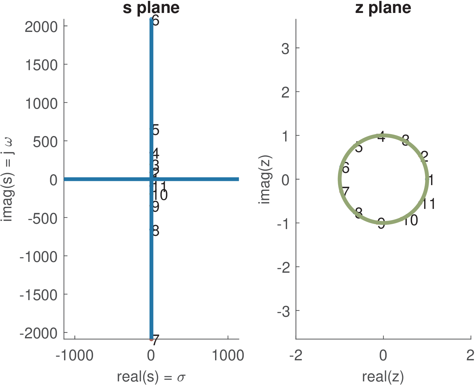
Figure 3.33(b) uses the same choice of points in z as in Figure 3.33(a), but now with $F_{s}$ increased from $8$ to 150 Hz. Comparing these two figures, one can notice that the same point “6” in plane z leads to $s = j ω_{0}$ where $ω_{0}$ is larger than 2000 rad/s in Figure 3.33(b) and less than 120 rad/s in Figure 3.33(a).

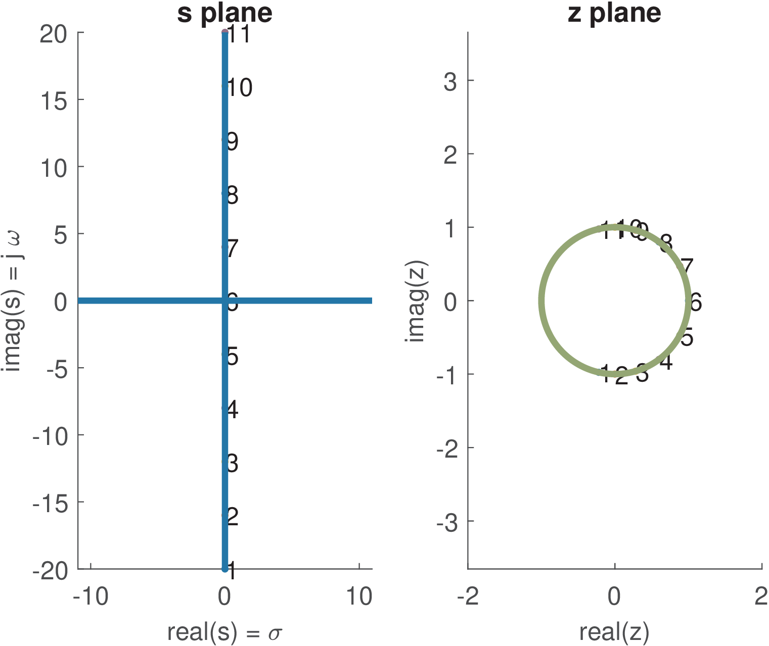
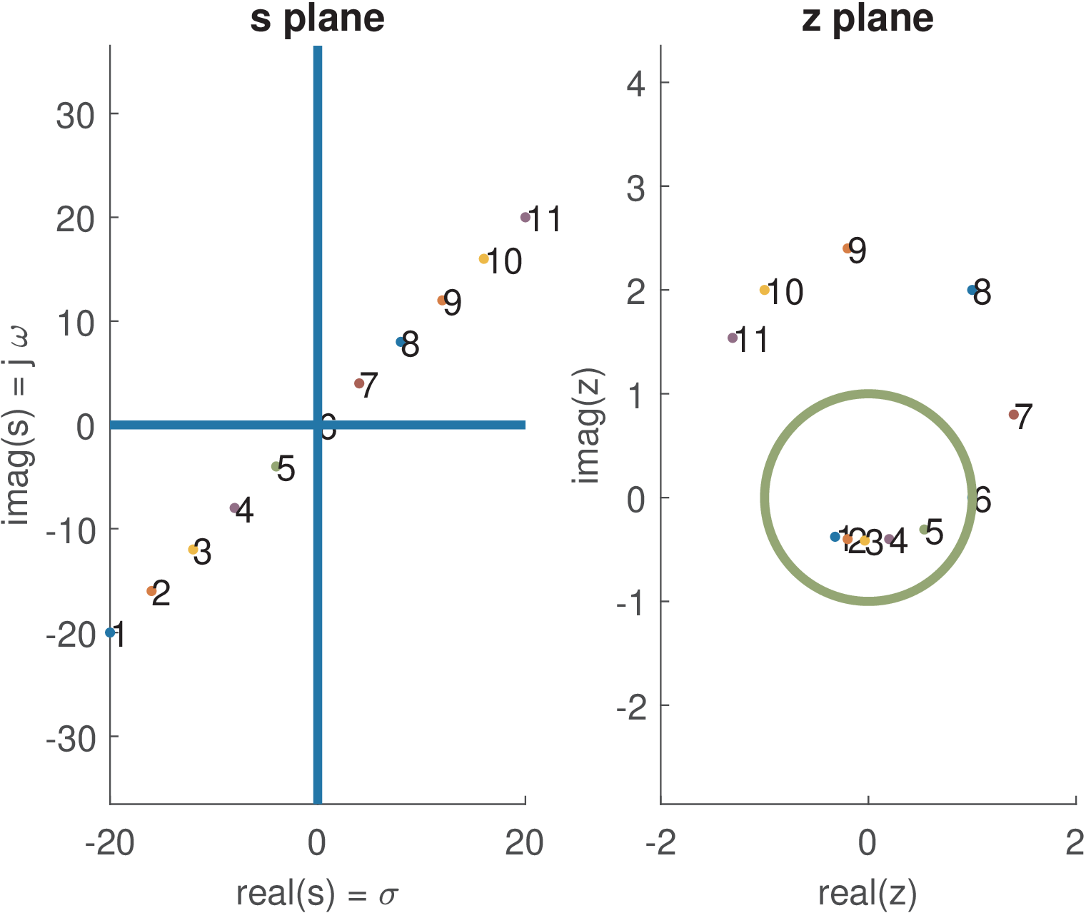
Figure 3.33(c) shows that the points in $s = jω$ are mapped into the z unit circle. Figure 3.33(d) illustrates that points at the left half S-plane are mapped inside the unit circle in z, while the points at the right half s plane are outside this circle. This fact explains the mentioned property of the bilinear transformation: causal and stable filters $H (s)$ are mapped to causal and stable filters $H (z)$ .

Careful observation of Figure 3.33(c) allows to conclude that a linear spacing among the points in the s plane corresponds to a non-linear spacing in the z plane. This fact is further studied in the next subsection.

3.12.2 Non-linear frequency warping imposed by bilinear

Assume the bilinear transformation was used to map $H_{s} (s)$ into $H_{z} (z)$ (the subscripts will make easier to distinguish the two transfer functions). The current task is to observe the relation between frequencies $Ω$ and $ω$ in the discrete and continuous-time, respectively, when the bilinear is used. This mapping between $Ω$ and $ω$ was illustrated in Figure 3.33(a) to Figure 3.33(c).

By the definition of bilinear in Eq. (3.64), the mapping between the frequency responses can be found by substituting $s = jω$ and $z = e^{j Ω}$ into Eq. (3.72). This leads to

jω = \frac{2 (e^{j Ω} - 1)}{T_{s} (e^{j Ω} + 1)} = \frac{2 j sin (Ω ∕ 2)}{T_{s} cos (Ω ∕ 2)},

(3.74)

where the second equality follows from the tricks of Eq. (A.14) and Eq. (A.15) applied to numerator and denominator, respectively. Consequently, Eq. (3.74) can be written as

ω = \frac{2}{T_{s}} tan (\frac{Ω}{2}) = 2 F_{s} tan (\frac{Ω}{2}),

(3.75)

which indicates how the bilinear relates $ω$ (rad/s) and $Ω$ (rad). When the bilinear transformation relates $H (z)$ and $H (s)$ , the system function $H (z)$ behaves at frequency $Ω$ in the same way that $H (s)$ behaves at frequency $ω$ .

In spite of this nonlinear frequency warping imposed by the tangent in Eq. (3.75), the “shape” of $H (z)$ is typically a good approximation of $H (s)$ . For example, the ripples are maintained. In particular, “equal ripple” filters such as Chebyshev and elliptic have the ripples preserved.

As mentioned, an arbitrary $H (s)$ such as a differentiator (see its mask in Figure 3.47) may get severely distorted when converted to $H (z)$ using the bilinear transformation. Hence, the bilinear is the most used in practice to design the conventional lowpass, highpass, bandpass and bandstop IIR filters, which aim at a flat magnitude over the passband.

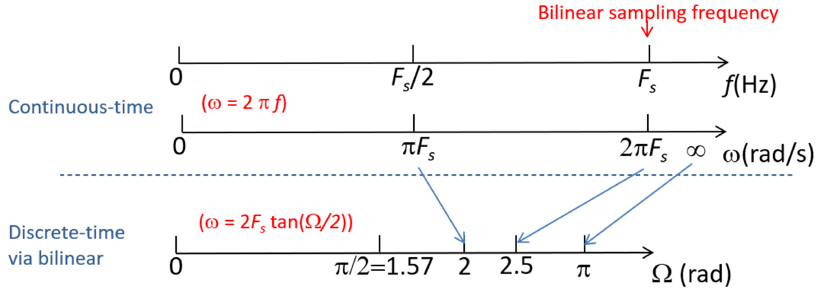
Figure 3.34: Version of Figure 1.45 in which the mapping between $ω$ and $Ω$ uses the bilinear transformation instead of the fundamental equation $ω = Ω F_{s}$ of Eq. (1.36).

From Eq. (3.75), it can be shown that the sampling ( $F_{s}$ ) and Nyquist ( $F_{s} ∕ 2$ ) frequencies, are mapped approximately to the digital frequencies $Ω = 2.5$ and 2 rad, respectively. This is illustrated in Figure 3.34. When $ω \to \infty$ , it is mapped by the bilinear into $Ω = π$ rad. In summary, the specific values $0, F_{s} ∕ 2, F_{s}, \infty$ of the continuous-time frequency $f = ω ∕ (2 π)$ are mapped, respectively into $Ω = 0, 2, 2.5$ and $π$ .

Note that $ω = Ω F_{s}$ (Eq. (1.36)), represented in Figure 1.45, is used when mapping from continuous-time to discrete-time via periodic sampling. The mapping between $ω$ and $Ω$ illustrated in Figure 3.34 is imposed by the bilinear transformation and happens in a very distinct situation: when using Eq. (3.64) to convert $H (s)$ into $H (z)$ . Some examples are provided in the next paragraphs to illustrate the bilinear frequency warping.

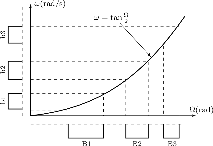
Example 3.24. Nonlinear relation among frequencies obtained with the bilinear transformation. Figure 3.35 illustrates the plot obtained with Listing 3.23, which assumes $F_{s} = 0.5$ Hz. Note that the three passbands have the same bandwidth in $ω$ ( $b_{1} = b_{2} = b_{3} = 0.4$ rad/s), but the bilinear mapping generates three distinct corresponding bandwidths $B_{1} > B_{2} > B_{3}$ in $Ω$ . The “nonlinear warping” that led to different bandwidths, would also occur in the other way around: considering a situation with equal bandwidths in $Ω$ .

Figure 3.35: Bilinear leads to a nonlinear warping between $ω$ (rad/s) and $Ω$ (rad). This example uses $F_{s} = 0.5$ Hz such that $ω = tan (Ω ∕ 2)$ .

Listing 3.23: MatlabOctaveCodeSnippets/snip_systems_bilinearmap.m. [ Python version]

1%% Plot the bilinear frequency relation 
2Fs=0.5; %sampling frequency. Use a convenient value. 
3W=linspace(0,3*pi/4,100); %digital frequencies in rad 
4w=2*Fs*tan(W/2); %analog (warped) frequencies in rad/s 
5plot(W,w), xlabel('\Omega (rad)'), ylabel('\omega (rad/s)') 
6%% Same bandwidths in w (rad/s) lead to decreasing bands in W (rad) 
7deltaw=0.4; w=[0.2+(1:6)*deltaw]; %frequencies in w (rad/s) 
8disp(['b1,b2,b3=' num2str(deltaw) ' rad/s (all have same value)']) 
9W=2*atan(w/(2*Fs)); %find the corresponding frequencies in W (rad) 
10disp(['B1,B2,B3=' num2str(W(2)-W(1)) ', ' num2str(W(4)-W(3)) ', ' ... 
11    num2str(W(6)-W(5)) ' rad, respectively']);

More specifically, executing Listing 3.23 leads to:

b1,b2,b3=0.4 rad/s (all have same value)
B1,B2,B3=0.48996, 0.2263, 0.11891 rad, respectively

which confirms the nonlinear frequency warping indicated in Figure 3.35. $□$

Example 3.25. Example of how frequencies $Ω$ and $ω$ are warped when related via the bilinear transformation. The warping of Eq. (3.75) is illustrated in Figure 3.36 for $F_{s} = 100$ Hz.

Figure 3.36: Relation imposed by the bilinear transformation between $ω$ (rad/s) and $Ω$ (rad) for $F_{s} = 100$ Hz. In this case, the frequency $ω_{0} = 540.4$ rad/s is mapped to $Ω_{0} = 2.433 \pm k 2 π$ rad.

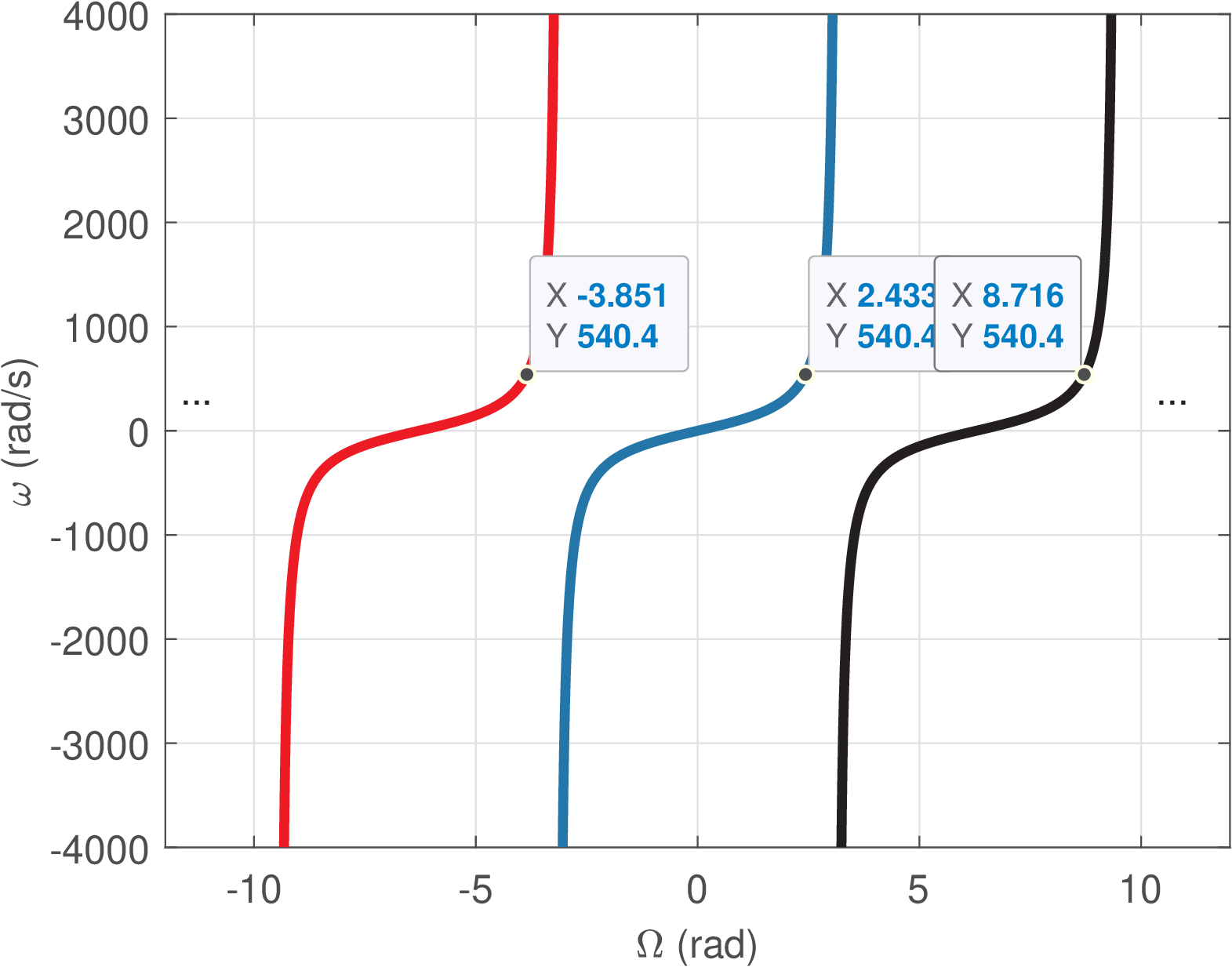
For instance, with $F_{s} = 100$ Hz, a given continuous-time angular frequency $ω_{0} = 540.4$ rad/s is mapped into $Ω_{0} = 2.433$ rad (or equivalently the multiples $Ω_{0} \pm k 2 π, k \in ℤ$ ), i. e., $H_{s} (540.4) = H_{z} (e^{j (2.433 \pm k 2 π)})$ . Figure 3.36 shows the discrete-time frequencies (angles) $Ω$ corresponding to $k = - 1, 0, 1$ .

Using the plot for $k = 0$ , $ω_{s} = 2 π F_{s} = 2 π 100 \approx 628.3$ rad/s is mapped, as expected from Eq. (3.75), to $Ω \approx 2.5$ rad. As discussed, the bilinear maps frequencies from $f = [0, F_{s}]$ Hz to $Ω = [0, 2.5]$ rad, and $f > F_{s}$ to $Ω =] 2.5, π]$ rad. $□$

Example 3.26. Using 2-d and 3-d graphs to observe how the bilinear maps s and z planes. This is another example that indicates how $H (s)$ is mapped into the z-plane by the bilinear transformation. Consider the system function

H (s) = 101 (s^{2} - 2 s + 1) ∕ (s^{3} + 3 s^{2} + 103 s + 101),

(3.76)

which can be obtained using

1    Hs_num=101*poly([1 1]); 
2    Hs_den=poly([-1 -1+1j*10 -1-1j*10]);

and has $ω = 10$ rad/s as the highest pole frequency. The poles at $- 1 \pm j 10$ create a peak at $ω = 10$ rad/s, which has a frequency of $10 ∕ (2 π) \approx 1.6$ Hz as shown in Figure 3.37. This $H (s)$ was chosen because it is not a standard filter realization with a flat passband, as illustrated in Figure 3.37. It is not evident in Figure 3.37, but $| H (f) | = 0$ when $f \to \infty$ due to the asymptotic decay with $- 20$ dB per decade imposed by the denominator order being 3 while the numerator’s is 2.

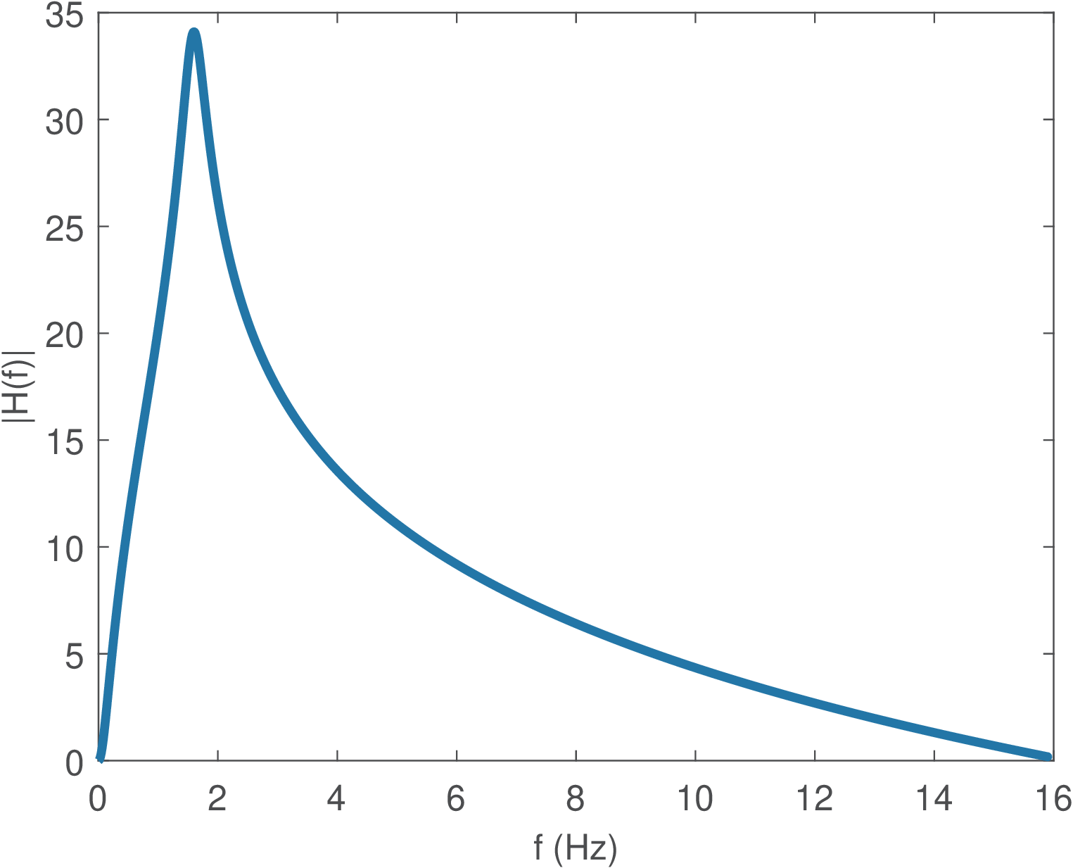
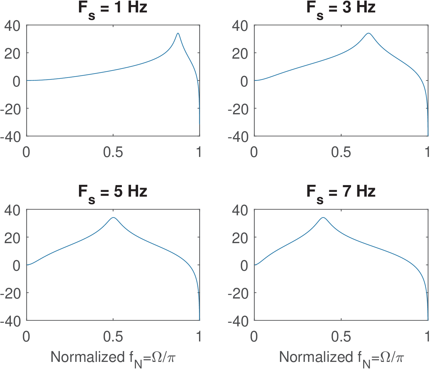
Figure 3.37: $| H (f) |$ corresponding to $H (s) = 101 (s - 1) (s - 1) ∕ [(s + 1) (s + 1 - j 10) (s + 1 + j 10)]$ of Eq. (3.76), to illustrate the bilinear transformation.

Figure 3.38: Frequency responses from $H (z)$ obtained via the bilinear transformation of $H (s)$ in Eq. (3.76) using $F_{s} =$ 1, 3, 5 and 7 Hz.

Figure 3.38 shows the magnitude (in dB) of four frequency responses from distinct $H (z)$ obtained with the bilinear transformation of $H (s)$ using the following sampling frequencies $F_{s}$ : 1, 3, 5 and 7 Hz. The plots illustrate aspects such as that the behavior of $| H (f) |$ when $f \to \infty$ (goes to $- \infty$ in dB scale, in this case) is mapped to $Ω = π$ rad.

Comparing Figure 3.37 and Figure 3.38, one can observe that the bilinear transformation may impose severe modifications when converting the function from the s to the z plane. That should be expected because it is desired to map the infinitely long $jω$ axis into the unit circle $e^{j Ω}$ and, to accomplish that, the bilinear mapping corresponds to the nonlinear warping of $jω$ imposed by Eq. (3.75).

Observing Figure 3.38 for the extreme case of $F_{s} = 1$ Hz and recalling that $F_{s}$ is always mapped to approximately $Ω = 2$ rad, the pole peak at $f = 1.6 > F_{s}$ in Figure 3.37 is then mapped to $Ω \in] 2, π]$ rad. In this case, the linear increase with frequency of the magnitude in dB scale observed in $| H (f) |$ from $f = 0$ to 1.6 Hz is severely distorted in $| H (e^{j Ω}) |$ .

Figure 3.39: Magnitude (in dB) for bilinear transformations of $H (s)$ in Eq. (3.76) for $F_{s} = 1$ (top-left), 3 (top-right), 5 (bottom-left) and 7 Hz. The values that $H (z)$ assumes for the unit circle $| z | = 1$ are indicated by the black contours. The corresponding 2-d frequency response magnitudes are depicted in Figure 3.38.

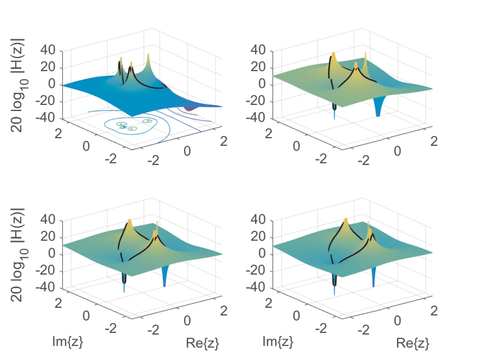
The 3-d plots of $| H (z) |$ for the whole Z plane can further illustrate the impact of $F_{s}$ in the bilinear transformation. The function ak_bilinearPlotZPlane.m was used to obtain Figure 3.39. Given $H (s)$ , varying $F_{s}$ locates the three poles in different positions. While for $F_{s} = 1$ Hz the pair of complex-conjugate poles have angles closer to $\pm π$ rad, the angles move towards 0 when $F_{s}$ increases, such that they are approximately $\pm π ∕ 2$ rad when $F_{s} = 5$ Hz. This 3-d view complements the information in Figure 3.38. $□$

3.12.3 Tracking the frequency warping provoked by bilinear

The next paragraphs discuss how the frequencies $ω_{c}$ of a continuous-time filter $H (s)$ are warped by Eq. (3.75) and mapped into frequencies $Ω$ of discrete-time $H (z)$ , and then mapped back to continuous-time frequencies $ω_{d}$ when using Eq. (1.36). Hence, one is dealing with two frequency normalizations: $ω = \frac{2}{T_{s}} tan (\frac{Ω}{2})$ , which is imposed by the bilinear, and $ω = Ω F_{s}$ , which is due to the uniform sampling.²⁵

Therefore, when an IIR filter $H (z)$ is designed using $H (s)$ as starting point and later implemented in a system with sampling frequency $F_{s}$ , there are three frequency categories of interest:

$ω_{a}$ : the analog angular frequencies associated to the analog filter $H (s)$ ,
$Ω$ : the digital frequencies of $H (z)$ (or $H (e^{j Ω})$ )
$ω_{d}$ : other analog frequencies, which are related to $Ω$ via $ω = F_{s} Ω$ as indicated in Eq. (3.26).

It is useful to adopt a more elaborated notation to relate these frequencies to their corresponding frequency responses. With this goal, the system functions $H (s)$ and $H (z)$ will be denoted as $H_{s} (s)$ and $H_{z} (z)$ , respectively.

As used before, the frequency response of the analog filter is $H_{s} (ω_{a})$ , while $H_{z} (e^{j Ω})$ is adopted for the digital filter. When $H_{z} (z)$ is followed by a D/S step as in Eq. (3.26), the equivalent frequency response of this combined action will be denoted here as $H_{z} (e^{j ω_{d} T_{s}})$ . The subscripts of $ω_{a}$ and $ω_{d}$ suggest: from “analog” and “digital” filters, respectively (they are both “analog” frequencies, in rad/s, such that $ω_{d}$ is not a digital frequency).

When dealing with the bilinear transformation and knowing the $F_{s}$ value that will be used, it is then useful to rewrite Eq. (3.75) using $ω_{d} = F_{s} Ω$ (as it was done to obtain Eq. (3.24)), which leads to

ω_{a} = \frac{2}{T_{s}} tan (\frac{T_{s} ω_{d}}{2}) .

(3.77)

Eq. (3.77) indicates that, when the bilinear transformation is adopted, $H (s)$ behaves at frequency $ω_{a}$ in the same way that the continuous-time equivalent version of $H (z)$ behaves at frequency $ω_{d}$ . In other words, the two systems have the same gain and phase at frequencies $ω_{a}$ and $ω_{d}$ , respectively. The goal of the next example is to expose this relation.

Example 3.27. Frequencies $ω_{a}$ and $ω_{d}$ in bilinear warping. As an example of analog system, Listing 3.24 obtains

H_{s} (s) = \frac{- 13600 (s - 1)}{s^{5} + 4.2 s^{4} + 421.81 s^{3} + 1638.2 s^{2} + 8407 s + 13600}

(3.78)

and converts it to $H_{z} (z)$ using bilinear. The filter $H_{s} (s)$ is lowpass and its pole with highest frequency is at $ω = 20$ rad/s, which is $f = 20 ∕ (2 π) \approx 3.2$ Hz. The adopted sampling frequency was $F_{s} = 10$ Hz.

Listing 3.24: MatlabOctaveCodeSnippets/snip_systems_sampling.m

1a=1; %zeros in the s-plane 
2b=-2; c=-1+1j*4; d=-0.1+1j*20; %poles in the s-plane 
3Hs_num=poly(a); %numerator of H_s(s) 
4Hs_den=poly([b c conj(c) d conj(d)]) %H_s(s) denominator 
5k=Hs_den(end)/Hs_num(end); %calculate factor 
6Hs_num=k*Hs_num %force a gain=1 at DC (s=0) 
7Fs=10; %sampling frequency (Hz) 
8[Hz_num, Hz_den] = bilinear(Hs_num, Hs_den, Fs) %bilinear

Figure 3.40 shows²⁶ the magnitude of frequency responses of (from top to bottom) $H_{s} (ω_{a})$ , $H_{z} (e^{j Ω})$ and $H_{z} (e^{j ω_{d} T_{s}})$ .

Note that the frequency axis of $H_{z} (e^{j Ω})$ has been warped²⁷ according to Eq. (3.77).

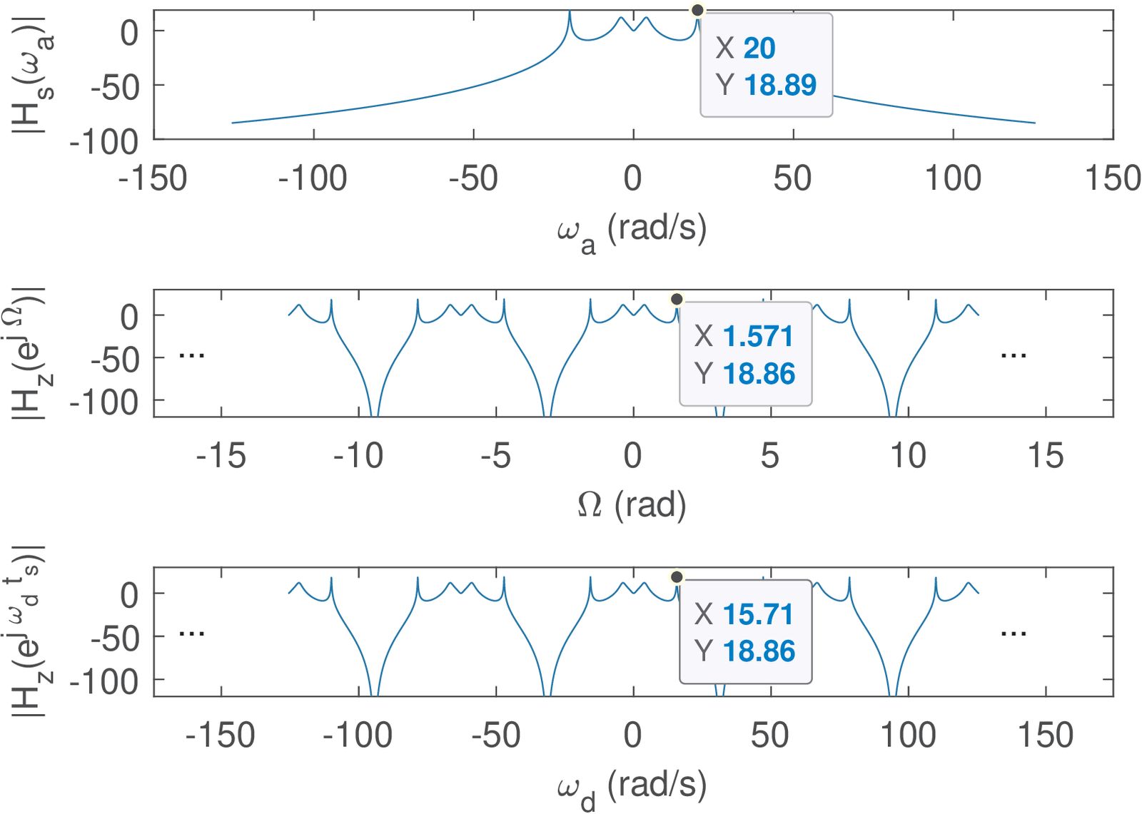
Figure 3.40: Frequency responses of $H_{s} (ω_{a})$ given by Eq. (3.78), $H_{z} (e^{j Ω})$ obtained via bilinear with $F_{s} = 10$ Hz and $H_{z} (e^{j ω_{d} T_{s}})$ (from top to bottom). Note that the intrinsic bilinear frequency warping converts $ω_{a} = 20$ rad/s into $ω_{d} = 15.71$ rad/s.

The pole at $ω_{a} = 20$ rad/s was mapped to

ω_{d} = \frac{2}{T_{s}} {tan}^{- 1} (\frac{T_{s} ω_{a}}{2}) = \frac{2}{0.1} {tan}^{- 1} (\frac{0.1 \times 20}{2}) \approx 15.71 rad/s,

which can be checked via the commands:

1wa=20; Ts=1/10; wd=2/Ts*atan(Ts*wa/2)

In some situations, it is desirable to avoid that a frequency of interest ( $ω_{a} = 20$ rad/s in this case) becomes mapped to another frequency $ω_{d} \neq ω_{a}$ . In such cases, a pre-warping procedure can be adopted, as will be discussed in Section 3.13.1. $□$

3.12.4 Advanced: Properties of the bilinear transformation

The bilinear transformation has two important properties for digital filtering applications:

it is capable of maintaining the order of $H (z)$ equals to the order of the original proper $H (s)$ , and
if $H (s)$ is causal and stable, then so it is $H (z)$ .

It has also other interesting properties. The bilinear makes any point in the s-plane to be mapped onto a unique point in the z-plane and vice-versa. It establishes a correspondence between the “analog” DC $s = 0$ and the “digital” DC $z = 1$ . Similarly, it maps the highest digital frequency $Ω = π$ into the highest analog frequency $s = j∞$ .

The bilinear transformation generates $H (z)$ with the same number of poles as in $H (s)$ . In fact, a finite pole or zero at $s = s_{0}$ is mapped to a pole or zero at

z = \frac{2 + T_{s} s_{0}}{2 - T_{s} s_{0}} .

(3.79)

From Example 3.21, one can check that s=-2+j;Ts=0.1;z=(2+Ts*s)/(2-Ts*s) outputs 0.81 + 0.082j, as indicated in Eq. (3.66).

If $T_{s}$ is too small (make $T_{s} \to 0$ in Eq. (3.79)), the bilinear maps the pole (or zero) into $z = 1$ , which can significantly distort the original $H (s)$ . On the other hand, if $T_{s} \to \infty$ , it would be mapped to $z = - 1$ .

As depicted in Figure 3.41, when the bilinear is used for designing IIR filters, the value of $T_{s}$ is used twice and cancels out. In these cases, an arbitrary and reasonable (not too large or small) value such as $T_{s} = 1$ can be used. In cases in which $T_{s}$ does not cancel out (e. g., in some designs of a digital controller), it is important to choose a value that preserves in $H (z)$ the characteristics of interest in $H (s)$ .

The bilinear can create extra zeros at $z = - 1$ . This behavior can be studied by applying the bilinear transformation to $H (s) = 1 ∕ (s - s_{0})$ . For higher order $H (s)$ , most of the extra zeros at $z = - 1$ are canceled.²⁸

Another aspect is that, when mapping a given $H (s)$ to $H (z)$ using the bilinear, their values can be forced to match at a single frequency value. For filters having a single cutoff frequency such as lowpass and highpass filters, this frequency is often the chosen one.

When using the bilinear, the values of $H (s)$ and $H (z)$ can coincide in only one frequency value, but when designing IIR filters, one can obtain $H (s)$ already taking in account that the bilinear will distort the frequencies. This can be done by “pre-warping” the frequencies of interest and is not limited to a single frequency. In other words, it is possible to use “pre-warping” in all frequencies of interest (e. g., passband and stopband frequencies for a lowpass) to obtain $H (s)$ and, after this stage, face the bilinear restriction of matching $H (s)$ and $H (z)$ in a single frequency.

²³ In spite of being a mapping (transformation) from $H (s)$ to $H (z)$ , calling it “bilinear transform” is common in the DSP jargon.

²⁴ This derivation is just illustrative and the bilinear can also be obtained by applying trapezoidal numerical integration. See alternatives in Problem 3.4.

²⁵ Both $ω_{c}$ and $ω_{d}$ are given in radians per second, while $Ω$ is given in radians.

²⁶ Note that Figure 3.40 is an extended version of Figure 3.15. The same frequency responses were used and only the y-axis ranges differ.

²⁷ And, consequently, the axis of $H_{z} (e^{j ω_{d} T_{s}})$ too, given that it is obtained via a simple linear scaling $Ω = ω_{d} T_{s}$ .

²⁸ Inspect the source code of a bilinear function to check the algorithm that deals with this cancellation. For instance, look at function normalize called by Python’s bilinear at [ url3bin].