Relating Frequencies of Continuous and Discrete-Time Signals

1.8 Relating Frequencies of Continuous and Discrete-Time Signals

When periodic sampling is used with sampling frequency $F_{s}$ , the frequencies that show up in $x (t)$ are mapped into frequencies in $x_{s} (t)$ and $x [n]$ . This section discusses such mappings. We start by observing that angular frequencies are denoted as $ω$ and $Ω$ , in continuous and discrete-time, respectively. This notation is important because they have different units and properties.

1.8.1 Units of continuous-time and discrete-time angular frequencies

In essence, a continuous-time signal (for instance, $x (t) = cos (ωt)$ ) has radians per second (rad/s) as the unit of the angular frequency $ω$ . Multiplying $ω$ by $t$ , which is given in seconds, leads to an angle in radians. In contrast, the unit of the angular frequency $Ω$ of a discrete-time signal (for instance, $x [n] = cos (Ω n)$ ) is given in radians. Because $n$ is dimensionless, $Ω n$ is an angle in radians. Similar to the interpretation of discrete-time $n$ as “time”, in spite of being an angle, $Ω$ will be interpreted as angular frequency.

The different units of $ω$ (rad/s) and $Ω$ (rad) will play a fundamental role in discrete-time signal processing: a function $f (ω)$ of $ω$ can assume distinct values when $ω$ is varied in the range $[- \infty, \infty]$ , while a function $f (Ω)$ is periodic if $Ω$ is an angle. More specifically, when the variable $Ω$ is used to denote a discrete-time angular frequency, any function $f (Ω)$ of $Ω$ will have a period of $2 π$ rad and be typically evaluated only in a range of $2 π$ , such as $[0, 2 π [$ or $[- π, π [$ .

In other words, whenever $Ω$ is an angular frequency (that is, an angle), the function $f (Ω) = f (Ω + 2 π), \forall Ω$ is periodic and $Ω$ shows up as the argument of cosines or sines. For example, $f (Ω) = cos (3 Ω) ∕ cos (5 Ω)$ and $f (Ω) = e^{j 2 Ω}$ are possible functions of an angular frequency $Ω$ . In fact, it is a common practice to use the notation $f (e^{j Ω})$ to indicate that $f$ is a function of an angle $Ω$ (see, e. g. Eq. (2.34)). Therefore, one will never find something like $f (e^{j Ω}) = (3 + Ω) ∕ (5 + Ω)$ because the periodicity $f (Ω) = f (Ω + 2 π)$ is not observed in this case.

1.8.2 Mapping frequencies in continuous and discrete-time domains

In the following paragraphs, the main goal is not to prove, but to motivate the fundamental equation

ω = Ω F_{s},

(1.36)

where $F_{s}$ is the sampling frequency assumed to be in Hertz, $ω$ is the continuous-time angular frequency given in radians per second and $Ω$ is the discrete-time angular frequency given in radians.

To better interpret Eq. (1.36), one can apply the S/D conversion to a single sinusoid, as exemplified in the next paragraphs.

Example 1.34. Example of using the fundamental equation for relating angular frequencies of continuous-time and discrete-time cosines. Assume $x (t) = 10 cos (24 πt)$ is sampled with sampling interval $T_{s}$ to create the signal $x_{s} (t)$ via the impulse sifting property of Eq. (1.31):

x_{s} (t) = \sum_{n = - \infty}^{\infty} 10 cos (24 πn T_{s}) δ (t - n T_{s}) .

(1.37)

In this case, the S/D conversion of $x_{s} (t)$ results in

x [n] = S/D {x_{s} (t)} = 10 cos (24 π T_{s} n) = 10 cos (\frac{24 π}{F_{s}} n) .

Note that the original angular frequency $ω = 24 π$ radians/s was converted to the angular frequency in discrete-time $Ω = 24 π ∕ F_{s}$ radians, which corresponds to $Ω = ω ∕ F_{s}$ in Eq. (1.36).

For example, assuming $F_{s} = 36$ Hz, the cosine with angular frequency $ω = 24 π$ rad/s (that is equivalent to the linear frequency $f = 12$ Hz in this case) will be mapped to the angle $Ω = 2 π ∕ 3$ rad. Using Eq. (1.36) in the other direction, a discrete-time angular frequency of $Ω = π$ rad is always mapped to $ω = π F_{s}$ . In the given example, $Ω = π$ rad is mapped into $ω = 36 π$ rad/s or, equivalently, $f = 18$ Hz. $□$

The previous example can be generalized. In summary, Eq. (1.36) is valid for all pairs of continuous-time and discrete-time signals that are related by a C/D or D/C conversion obtained with periodic sampling.

Example 1.35. Another example of conversion between discrete and continuous-time domains. Assume a discrete-time signal $x [n] = 10 cos ((2 π ∕ 7) n)$ . It is possible to indicate that its angular frequency is $Ω = 2 π ∕ 7$ rad because the signal repeats itself every $N = 7$ samples. However, because $n$ is dimensionless, there is no information about time in this case. If it is stated that $x [n]$ was obtained via sampling at $F_{s} = 10$ Hz, $x [n]$ would be representing a cosine of angular frequency $ω = 20 π ∕ 7$ rad/s. Instead, if $F_{s} = 100$ Hz, then $ω = 200 π ∕ 7$ rad/s. As indicated in Eq. (1.36), the sampling frequency is needed when mapping the discrete-time angular frequency $Ω$ into the corresponding continuous-time angular frequency $ω$ . $□$

In summary, $F_{s}$ in Eq. (1.36) plays the role of a normalization factor that relates angular frequencies of continuous-time signals and their discrete-time counterparts obtained by C/D conversion. It leads to two distinct ways of simulating a continuous-time sinusoid using a discrete-time signal.

Example 1.36. Two approaches to simulate continuous-time sinusoids. Listing 1.14 indicates how to use Eq. (1.36) to create discrete-time sinusoids. The task is to generate a cosine of 600 Hz using Matlab/Octave. Two distinct approaches are:

f 1.: use “continuous-time” frequencies $f$ (in Hz) or $ω$ (in rad/s), with discretized time $t$ in seconds, or
f 2.: use “discrete-time” frequencies $Ω$ (in rad), obtained via Eq. (1.36), and using a dimensionless “time” $n$ .

These two approaches are contrasted in Listing 1.14.

Listing 1.14: MatlabOctaveCodeSnippets/snip_signals_sinusoid_generation.m. [ Python version]

1Fs=8000; %sampling frequency (Hz) 
2Ts=1/Fs; %sampling interval (seconds) 
3N=20000; %number of desired samples 
4f0=600; %cosine frequency (Hz) 
5%%%%First alternative to generate a cosine of 600 Hz 
6t=0:Ts:(N-1)*Ts; %discretized continuous-time axis (sec.) 
7x1=5*cos(2*pi*f0*t); %amplitude=5 V and frequency = f0 Hz 
8%%%%Second alternative: work directly in discrete-time 
9w0=2*pi*f0*Ts; %w0 is in rad, convert from rad/s to rad 
10n=0:N-1; %discrete-time axis (do not use Ts anymore) 
11x2=5*cos(w0*n); %amplitude=5 V and frequency = w0 rad 
12plot(x1-x2); %plot error between two alternative sequences 
13soundsc(x1,Fs) %for fun: playback one of them to listen

Note that the sequences x1 and x2 are essentially the same, and there are only small numerical errors. In essence, one can simulate discrete-time signals representing the time evolution either with $n$ (an integer) or $t$ (in seconds), but properly using the corresponding angular frequencies $Ω$ (in radians) or $ω$ (in rad/s), respectively.

Listing 1.14 compared signals created with $n = 0, 1, 2, \dots,$ versus $t = n T_{s} = 0, 125 \times 1 0^{- 6}, 250 \times 1 0^{- 6}, \dots,$ (given that $T_{s} = 1 ∕ F_{s} = 125 \times 1 0^{- 6}$ seconds), with the corresponding angular frequencies being $Ω = 2 π 600 ∕ 8000 \approx 0.471$ rad or $ω = 2 π 600 \approx 3769.9$ rad/s, respectively. $□$

1.8.3 Nyquist frequency

As indicated by Eq. (1.30), if the sampling theorem is obeyed, the maximum frequency in the original continuous-time signal $x (t)$ is restricted to $f_{max} < F_{s} ∕ 2$ Hz, where $F_{s} ∕ 2$ is called the Nyquist frequency.

Using Eq. (1.36), one can see that angle $Ω = π$ rad will be mapped into $ω = Ω F_{s} = π F_{s}$ rad/s, which corresponds to the Nyquist frequency $F_{s} ∕ 2$ Hz. This is consistent with the fact that $π$ represents the highest frequency in discrete-time processing. This can be observed by plotting $x [n] = cos (Ω n)$ and varying $Ω$ until it reaches $π$ rad, which corresponds to a period of $N = 2$ samples. Increasing $Ω$ from $π$ to $1.5 π$ , for instance, will slow down the signal (observe the angles: $1.5 π = - 0.5 π$ ), and increase the period to $N = 4$ samples.

1.8.4 Frequency normalization in Python and Matlab/Octave

It is sometimes inconvenient to show graphs with the abscissa using $Ω$ in radians. For example, a graph in the range $[0, π]$ would have the last abscissa value as approximately $3.14159$ , which could be annoying. To avoid that, the convention adopted by Matlab/Octave is to use, instead of $Ω$ in rad, a normalized frequency

f_{N} = Ω ∕ π .

(1.38)

This division by $π$ maps the discrete-time angular frequency range $[0, π]$ rad into the range $[0, 1]$ of a normalized frequency $f_{N}$ .

Given the sampling frequency $F_{s}$ and the fact that $Ω = ω ∕ F_{s}$ (from Eq. (1.36)), Eq. (1.38) can be conveniently written as

f_{N} = \frac{Ω}{π} = \frac{ω}{F_{s} π} = \frac{2 πf}{F_{s} π} = \frac{f}{F_{s} ∕ 2} .

(1.39)

Having a frequency $f$ in Hz, Eq. (1.39) can be used to map it to $f_{N}$ in the range $[0, 1]$ as required by software such as Matlab/Octave and Python, and indicated in Eq. (1.38). For instance, if $F_{s} = 10$ Hz, a frequency $f$ =4 Hz after the sampling process would be represented as $f_{N} = 4 ∕ 5$ in Matlab/Octave or Python, which can be quickly calculated via

f_{N} = \frac{f}{F_{s} ∕ 2},

(1.40)

i. e., $f$ is simply divided by the Nyquist frequency $F_{s} ∕ 2$ .

Table 1.5: The notation and values of the Nyquist frequency in distinct domains.


$f$ (Hz)	$ω$ (rad/s)	$Ω$ (rad)	Matlab/Octave normalized $f_{N}$ ( $Ω ∕ π$ )

$F_{s} ∕ 2$	$π F_{s}$	$π$	1

Figure 1.45: Versions of the Nyquist frequency in continuous and discrete-time.

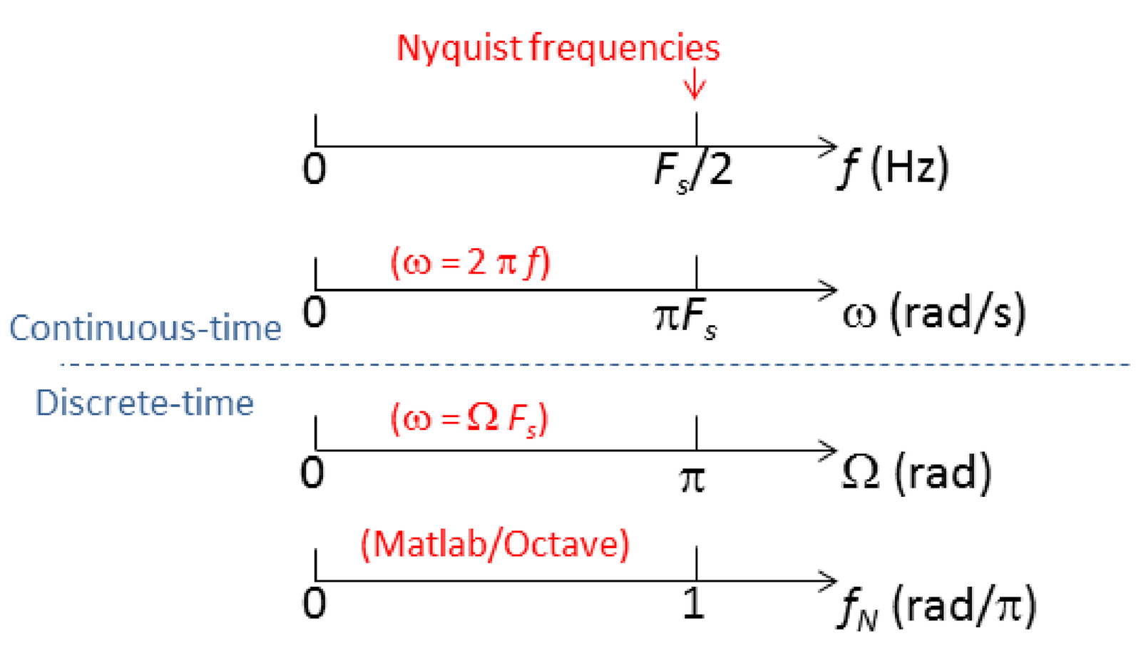
Table 1.5 and Figure 1.45 summarize the discussed information about versions of the Nyquist frequency in different domains, including its normalized version in Matlab/Octave. Figure 1.45 is also useful to observe the relation between the frequencies $ω$ , $f$ , $Ω$ and $f_{N}$ .