Modeling the Stages in A/D and D/A Processes

1.7 Modeling the Stages in A/D and D/A Processes

This section discusses mathematical models that are used to conveniently represent in a high-level, the individual signal processing stages in the A/D and D/A processes.

Different electronic circuits can be used when designing an ADC chip to perform the A/D process such as successive approximation and sigma-delta. If needed, the signal processing stages used in each of these techniques can be modeled with details. For instance, a detailed description may be necessary in case the goal is to optimize the electronic circuits to be more robust to impairments and noise. In the scope of this text, these details are not important and the A/D process is considered ideal. A similar approach is adopted for the D/A process.

1.7.1 Modeling the sampling stage in A/D

The goal here is to extract samples to represent an analog signal $x (t)$ . In periodic (or uniform) sampling of a continuous-time function $x (t)$ with a sampling interval $T_{s}$ , the sampling frequency is

F_{s} = \frac{1}{T_{s}} .

(1.25)

For example, digital telephony adopts $F_{s} = 8000$ Hz, which corresponds to $T_{s} = 125$ $μ$ s.

Figure 1.26: An impulse train with unitary areas and $T_{s} = 125$ $μ$ s.

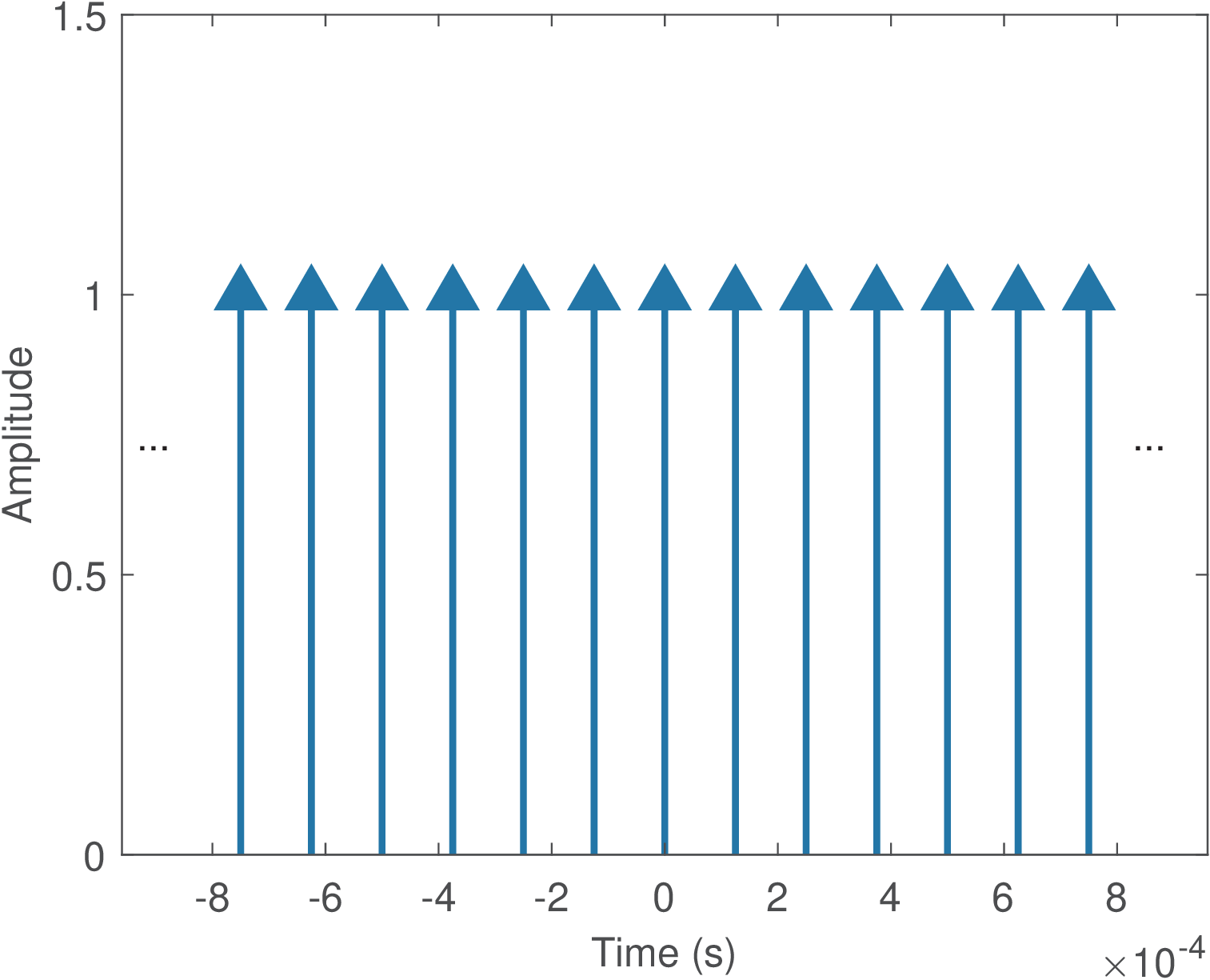
In the A/D context, periodic sampling can be modeled as the multiplication of $x (t)$ by a periodic impulse train $p (t)$ . Figure 1.26 depicts the infinite duration impulse train for sampling at 8 kHz. As conventionally done, the impulses heights indicate their areas. The sampled signal is denoted as

x_{s} (t) = x (t) p (t) = \sum_{k = - \infty}^{\infty} x (k T_{s}) δ (t - k T_{s}),

where $x (k T_{s})$ is the impulse area in $x_{s} (t)$ , which coincides with the amplitude of $x (t)$ at $t = k T_{s}$ . The amplitude of $x_{s} (t)$ is not defined when $t = k T_{s}$ (it goes to infinite, and only the area of the impulse is defined). And when $t \neq k T_{s}$ , the amplitude of $x_{s} (t)$ is zero. The notation $x_{s}^{area} (t)$ will sometimes be used to emphasize we mean the area of the impulse at time $t$ .

Example 1.22. Example of periodic sampling. Consider sampling the analog signal in Figure 1.1 via multiplying it by the train of impulses in Figure 1.26. Using the impulse sifting property (see Section A.26.5.0) leads to the sampled signal in Figure 1.15, which is depicted with the original analog signal superimposed.

In this case, the signal segment $x (t)$ in Figure 1.1 has $D = 6.125$ ms of duration. Given that $F_{s} = 8$ kHz, this segment is represented by $N = 50$ samples. To understand how $N$ is calculated in this case, observe that $x_{s} (t)$ starts and ends with samples, such that it contains $N - 1$ intervals of duration $T_{s} = 1 ∕ F_{s}$ with a total duration $D = (N - 1) T_{s} = (50 - 1) (1 ∕ 8000) = 6.125$ ms.

An alternative representation would be to assume that there are $N$ intervals of duration $T_{s}$ , such that $x_{s} (t)$ would end after an interval of $T_{s}$ seconds after its last impulse. One can find both representations in the literature and associated software. $□$

Figure 1.15 shows that, in this case, the sampled signal $x_{s} (t)$ represents very well the original analog signal $x (t)$ , in the sense that the envelope of the impulse areas correspond to a good match with respect to the original signal. This is not the case in the following example. Consider now that the sampling interval is increased by a factor of 4 to $T_{s} = 500 μ$ s. Figure 1.27 indicates that in this case $x_{s} (t)$ cannot represent well, for example, the variation between the samples indicated in the figure.

Figure 1.27: Example of a sampled signal obtained with a sampling frequency smaller than the required for accurately representing the original signal (shown in dotted lines).

In terms of computational cost, it is often convenient to use the smallest possible value of $F_{s}$ . But choosing $F_{s}$ too small may lead to a sampled signal that does not represent well the original signal as noted in Figure 1.27. Section 1.7.10 discusses a theorem that informs the minimum sampling rate for perfect reconstruction of a signal $x (t)$ from its samples $x [n]$ given the maximum frequency of $x (t)$ .

1.7.2 Oversampling

When the sampling rate $F_{s}$ is larger than the minimum required sampling rate, the signal is considered to be oversampled. Oversampling an analog signal may facilitate the consequent digital signal processing, especially when real-time is not a requirement. For instance, consider that a signal could be sampled with 8 kHz, but $F_{s} = 32$ kHz is adopted. If real-time processing is required, instead of processing 8,000 samples per second, now the system must process 32,000. In this case, the oversampling factor would be $L = 32, 000 ∕ 8, 000 = 4$ . Oversampling by a factor of $L$ , can also be interpreted as decreasing the sampling interval $T_{s} = 1 ∕ F_{s}$ by $L$ . For the given example, the interval $1 ∕ 8, 000 = 125$ $μ$ s between neighbor samples is reduced to $31.25$ $μ$ s.

In spite of the potential increase in computational cost of oversampling, it may be the case that higher accuracy can be obtained or eventually simpler algorithms adopted. It is very common to observe commercial DSP systems adopting $L = 2, 4$ or larger.

When simulating DSP in computers, a very large $L$ can be adopted to generate graphs of oversampled discrete-time signals that look like continuous-time signals.

Example 1.23. Mimicking continuous-time using discrete-time signals with a large oversampling factor. When representing a signal via a vector, one is implicitly dealing with a discrete-time signal. But even if a signal $x [n]$ is representing the samples of an analog signal $x (t)$ , sometimes it is desirable to generate graphs that resemble $x (t)$ . In such situations, one alternative is to use a large oversampling factor, as previously used in Listing 1.4. Listing 1.9 provides another example.

Listing 1.9: MatlabOctaveCodeSnippets/snip_signals_oversampling.m. [ Python version]

1Fs=8000; %sampling frequency (Hz) 
2Ts=1/Fs; %sampling interval (seconds) 
3f0=2400; %cosine frequency (Hz) 
4N=40; %number of desired samples 
5n=0:N-1; %generate discrete-time abscissa 
6t=n*Ts; %discretized continuous-time axis (sec.) 
7x=6*cos(2*pi*f0*t); %amplitude=6 V and frequency = f0 Hz 
8subplot(211), plot(t,x); %plot discrete-time signal 
9%% Create an oversampled version of signal x 
10oversampling_factor = 200; 
11oversampled_Ts = Ts/oversampling_factor; 
12oversampled_n = n(1)*oversampling_factor:n(end)*oversampling_factor; 
13oversampled_t=oversampled_n*oversampled_Ts;%oversampled discrete-time 
14xo=6*cos(2*pi*f0*oversampled_t); %oversampled discrete-time signal 
15subplot(212), plot(oversampled_t,xo);

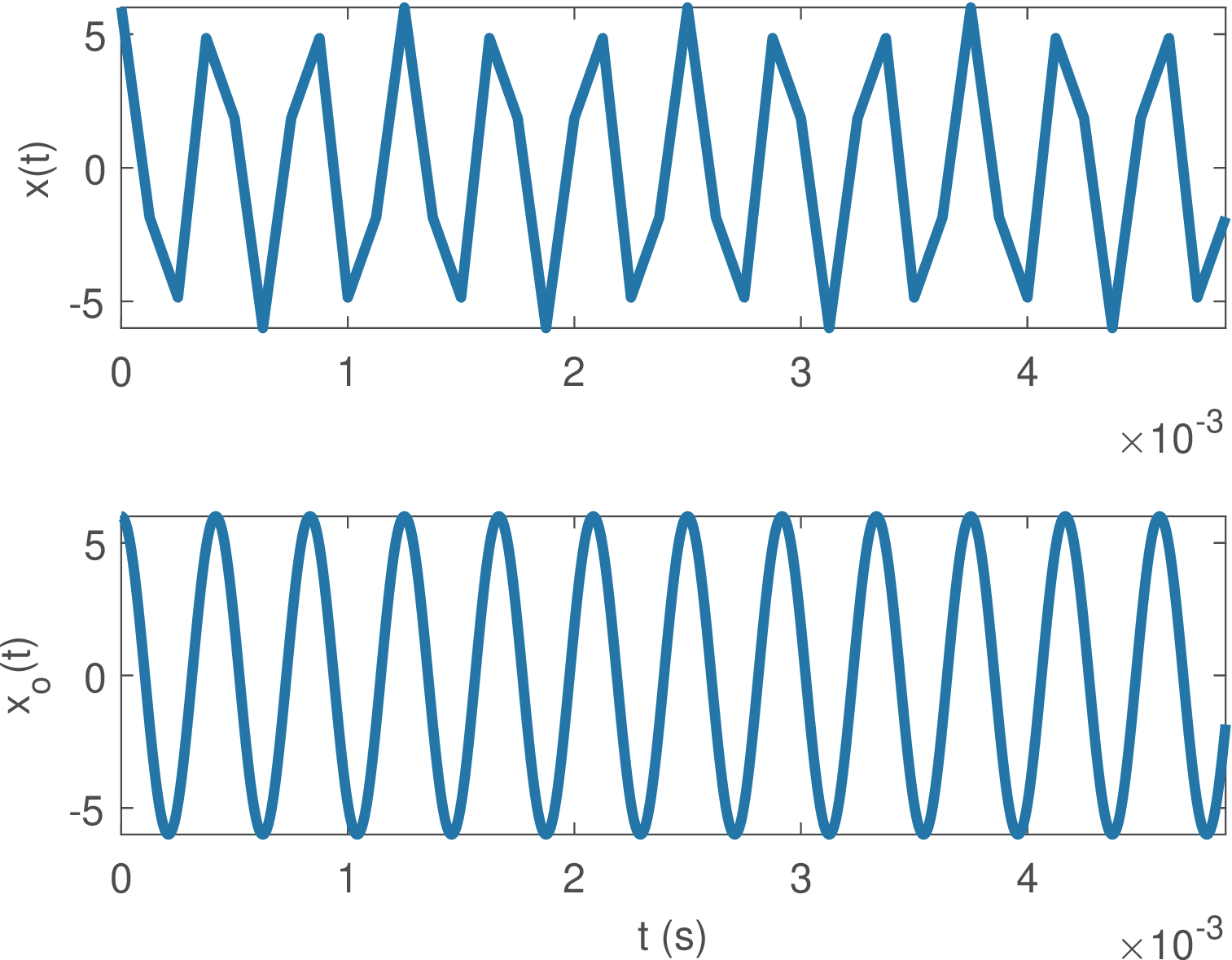
Figure 1.28: Example of discrete-time cosines generated with sampling intervals of $125$ $μ$ s (top) and 625 ns (bottom) to illustrate the better representation achieved by using a smaller sampling interval $T_{s}$ , which corresponds to adopting a larger oversampling factor.

Listing 1.9 generates x with a sampling interval $T_{s} = 1 ∕ 8, 000 = 125$ $μ$ s. It also creates an oversampled version xo using a new sampling interval of $T_{s} ∕ 200 = 625$ ns. Instead of using stem in Matlab/Octave, both graphs were generated with plot, assuming the goal is to depict a continuous-time signal. However, as can be seen in Figure 1.28, xo corresponds to a coarse representation of a cosine that uses $N = 40$ samples (length of x), while xo is a much better one using $N_{o} = 7801$ samples. $□$

There are several ways to create versions with different sample rates from a given signal $x (t)$ . In the specific case of Listing 1.9, the signals x and xo were created such that their first and last samples correspond to the same time instant, $t = 0$ and $t = 4.875$ ms, respectively. In this case, the number $N_{o}$ of samples in the oversampled xo is given by

N_{o} = L (N - 1) + 1,

(1.26)

where $N$ is the number of samples in x and $L$ is the oversampling factor. This equation can be understood by considering that xo has all $N$ samples of x plus the extra $L - 1$ samples between each of the $N - 1$ consecutive pairs of samples of x. This leads to $N_{o} = N + (L - 1) (N - 1)$ , which can be rewritten as Eq. (1.26).

When Eq. (1.26) is used for the signals in Listing 1.9, it leads to $N_{o} = 7801$ samples, as can be confirmed by the command length(x).

1.7.3 Mathematically modeling the whole A/D process

According to the convention adopted in this text, the following four signals appear during the A/D process along the stages of sampling (SAMPLING) and quantization (QUANTIZATION): analog, sampled, discrete-time and digital. Therefore, the A/D process is conveniently represented via the block diagram in Figure 1.29.

Figure 1.29: Complete process of A/D conversion with intermediate stages and four signals: analog, sampled, discrete-time and digital.

Figure 1.29 indicates that the sampled signals $x_{s} (t)$ is converted into the discrete-time signal $x [n]$ via the sampled to discrete-time (S/D) conversion. The sampling and S/D stages can be combined into the continuous to discrete-time (C/D) conversion. We first discuss the S/D conversion and then the C/D.

1.7.4 Sampled to discrete-time (S/D) conversion

The S/D conversion represents an intermediate stage in the periodic sampling process and is always associated to a given sampling interval $T_{s}$ . The actual signal processing performed by the electronic circuits of an ADC do not generate impulses or sampled signals, but the S/D conversion is a convenient mathematical model for the ideal periodic sampling. For example, if $x_{s} (t) = 3 δ (t + 2 T_{s}) - 1 δ (t + T_{s}) + 8 δ (t) - 5 δ (t - 3 T_{s})$ , the S/D conversion outputs $x [n] = 3 δ [n + 2] - 1 δ [n + 1] + 8 δ [n] - 5 δ [n - 3]$ .

Recall that $x_{s} (t)$ exists for all values of $t$ while $x [n]$ is a discrete time signal with $n \in ℤ$ . Another mathematical detail is that the non-zero amplitudes of $x_{s} (t)$ are $\pm \infty$ , but the corresponding areas $x_{s}^{area} (t)$ lead to the amplitudes of the corresponding $x [n]$ and are well-defined. For instance, $x_{s}^{area} (0) = 8$ and leads to the parcel $8 δ [n]$ in discrete-time.

Example 1.24. Example of S/D conversion. Figure 1.30 illustrates an example of S/D conversion assuming $T_{s} = 0.2$ s.

Figure 1.30: Example of S/D conversion assuming $T_{s} = 0.2$ s.

The visible samples of the input are $x_{s} (t) = 0.5 δ (t) - 2.8 δ (t - T_{s}) + 1.3 δ (t - 2 T_{s}) + 3.5 δ (t - 3 T_{s}) - 1.7 δ (t - 4 T_{s}) + 1.1 δ (t - 5 T_{s}) + 4 δ (t - 6 T_{s})$ . Their corresponding output values are $x [n] = 0.5 δ [n] - 2.8 δ [n - 1] + 1.3 δ [n - 2] + 3.5 δ [n - 3] - 1.7 δ [n - 4] + 1.1 δ [n - 5]) + 4 δ [n - 6]$ . $□$

1.7.5 Continuous-time to discrete-time (C/D) conversion

It is sometimes convenient to group the sampling and S/D stages into a single operation called continuous to discrete-time (C/D) conversion:

x (t) \to C ∕ D \to x [n] .

The only distinction between C/D and A/D conversions is that the former does not incorporate the quantization stage, as indicated in Figure 1.29.

1.7.6 Discrete-time to sampled (D/S) conversion

The discrete-time to sampled (D/S) conversion is basically the inverse of S/D. Figure 1.31 illustrates this, by depicting the inverse of the operation in Figure 1.30 of Example 1.24.

Figure 1.31: Example of D/S conversion assuming $T_{s} = 0.2$ s. It implements the inverse operation of Figure 1.30.

In Figure 1.31, the visible samples of the input are $x [n] = 0.5 δ [n] - 2.8 δ [n - 1] + 1.3 δ [n - 2] + 3.5 δ [n - 3] - 1.7 δ [n - 4] + 1.1 δ [n - 5]) + 4 δ [n - 6]$ . Giventhat $T_{s} = 0.2$ seconds, the corresponding output of the D/S conversion is $x_{s} (t) = 0.5 δ (t) - 2.8 δ (t - 0.2) + 1.3 δ (t - 0.4) + 3.5 δ (t - 0.6) - 1.7 δ (t - 0.8) + 1.1 δ (t - 1) + 4 δ (t - 1.2)$ .

While the S/D is a stage of the A/D process model, the D/S is part of the D/A.

1.7.7 Reconstruction

In the context of A/D and D/A processes, the sampling inverse operation is called reconstruction, and converts a sampled signal $x_{s} (t)$ into an analog signal $x (t)$ . Reconstruction is also called interpolation or filtering. It consists of choosing a function $h (t)$ that is combined with $x_{s} (t)$ as follows:

x (t) = \sum_{n = - \infty}^{\infty} x_{s}^{area} (n T_{s}) h (t - n T_{s}),

(1.27)

where $x_{s}^{area} (n T_{s})$ is the area of the impulse in $x_{s} (t)$ at time $t = n T_{s}$ .

The complete mathematical description of reconstruction will be discussed only in Section 3.5, after the concepts of convolution and filtering are presented.¹¹

Because $x_{s} (t)$ is obtained from $x [n]$ via a D/S process, it is convenient to rewrite Eq. (1.27) observing that the impulse area $x_{s}^{area} (n T_{s})$ coincides with its corresponding amplitude $x [n]$ , such that:

x (t) = \sum_{n = - \infty}^{\infty} x [n] h (t - n T_{s}) .

(1.28)

Eq. (1.28) indicates that $x (t)$ is obtained by shifting $h (t)$ by $t = n T_{s}$ , scaling this intermediate result by the corresponding amplitude $x [n]$ , and then summing up all these parcels.

Among many alternatives for choosing the reconstruction function $h (t)$ , two important ones are the so-called zero-order holder (ZOH) $h (t) = Π ((t - 0.5 T_{s}) ∕ T_{s})$ and sinc reconstruction $h (t) = sinc (t ∕ T_{s})$ . ZOH is useful for its simplicity, while sincs achieve a perfect reconstruction. They are discussed in the next paragraphs.

Reconstruction with zero-order holder (ZOH)

The ZOH consists of choosing $h (t)$ with amplitude 1 from $t = 0$ to $T_{s}$ . This can be written as $h (t) = Π ((t - 0.5 T_{s}) ∕ T_{s})$ (see Section 1.3.6). ZOH reconstruction sustains the amplitude of a given sample $x [n_{0}]$ (which coincides with the area $x_{s}^{area} (n_{0} T_{s})$ of the impulse at time $t = n_{0} T_{s}$ in signal $x_{s} (t)$ ) during an interval of $T_{s}$ seconds until the new sample $x [n_{0} + 1]$ updates this amplitude and so on.

Example 1.25. Example of ZOH reconstrucion. Eq. (1.28) implemented with ZOH is illustrated in Figure 1.32 for the signal $x_{s} (t)$ in Example 1.24. In this case, $T_{s} = 0.2$ s and, therefore, $h (t) = Π ((t - 0.5 T_{s}) ∕ T_{s}) = Π ((t - 0.1) ∕ 0.2)$ .

Figure 1.32: Example of ZOH reconstruction using the signals of Example 1.24 with $T_{s} = 0.2$ s. In this case, $x [n] = 0.5 δ [n] - 2.8 δ [n - 1] + 1.3 δ [n - 2] + 3.5 δ [n - 3] - 1.7 δ [n - 4] + 1.1 δ [n - 5]) + 4 δ [n - 6]$ .

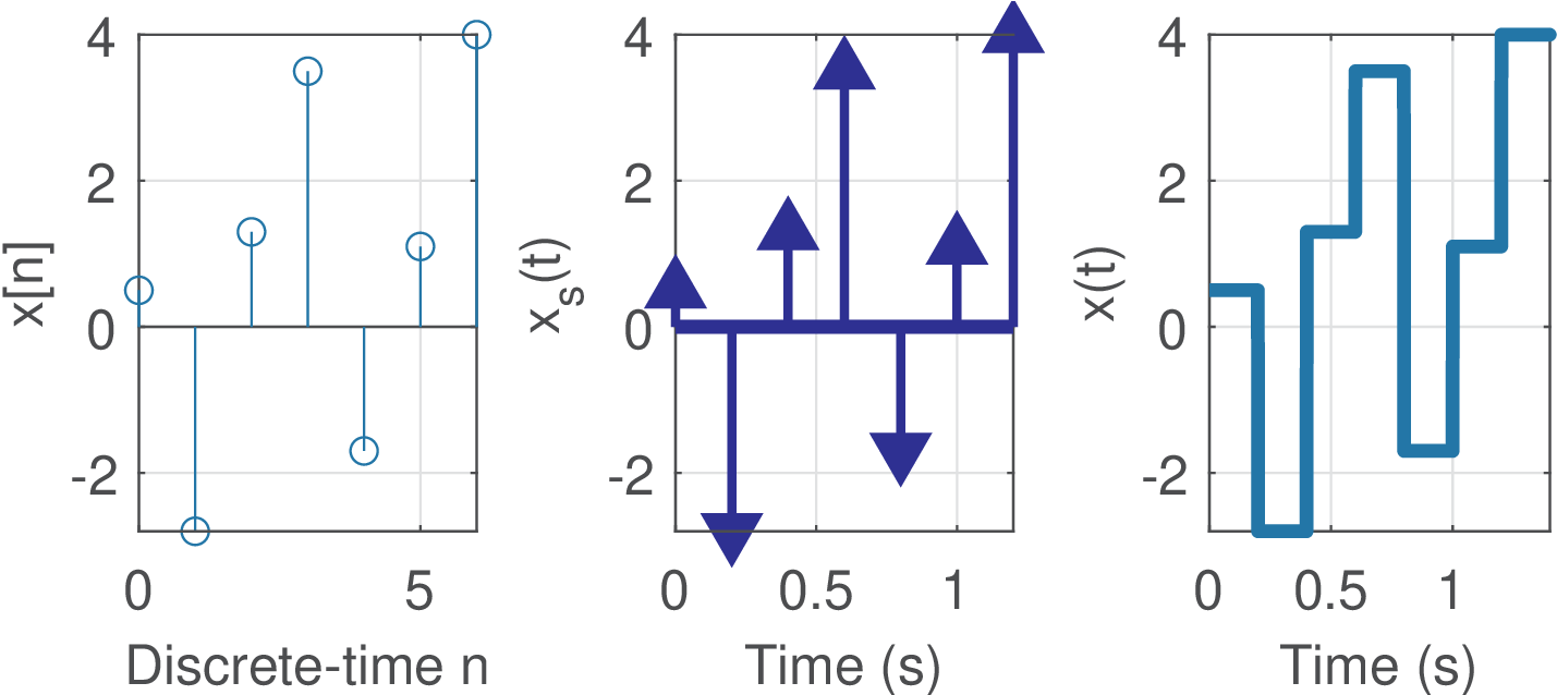
For instance, assuming $n_{0} = 0$ in Figure 1.32, the area of the impulse in $x_{s} (0)$ is 0.5 such that $x (t) = 0.5$ in the interval $t \in [0, T_{s} [$ . Then, in the interval $t \in [T_{s}, 2 T_{s} [$ the amplitude of $x (t)$ is $- 2.8$ , which is the area of the impulse at $x_{s} (T_{s})$ . And this “holding” process continues for other samples. $□$

Reconstruction with sincs

Reconstruction with sincs consists of choosing $h (t) = sinc (t ∕ T_{s})$ (see Figure 1.8). It is the ideal reconstruction, as will be discussed along with the sampling theorem when presenting Eq. (3.17).

Example 1.26. Perfect reconstruction with sinc functions. Figure 1.33 provides an example of Eq. (1.28) using sinc functions. In this case, $T_{s} = 0.2$ s and, therefore, $h (t) = sinc (t ∕ 0.2)$ .

Figure 1.33: Example of D/A of signal $x_{q} [n] = δ [n] - 3 δ [n - 1] + 3 δ [n - 2]$ (with quantized amplitudes) with D/S using $T_{s} = 0.2$ s and reconstruction using sinc functions.

The resulting signal $x (t)$ has an infinite support, extending from $t = - \infty$ to $\infty$ (Figure 1.33 depicts only the range $t \in [- 0.8, 0.8]$ ). It can be also noted that even $x_{q} [n]$ having quantized amplitudes, the reconstruction process creates an analog signal $x (t)$ for which the amplitudes assume an infinite number of different values.

Figure 1.34 provides more details about the bottom plot in Figure 1.33. Assuming $x_{q} [n]$ was obtained by sampling a continuous-time signal with the sampling theorem satisfied, this D/C conversion exactly recovers the original signal $x (t)$ .

In this case, the canonical $sinc (t)$ is contracted to $sinc (t ∕ T_{s}) = sinc (t ∕ 0.2) = sinc (5 t)$ , which has zeros at $t = \pm 0.2, \pm 0.4, \dots$ . Still as indicated in Eq. (1.28), the amplitude $x [n_{0}]$ at discrete-time $n_{0}$ multiplies the corresponding contracted and time-shifted $sinc (\frac{t - n_{0} T_{s}}{T_{s}})$ to create a parcel that is represented by a specific color and dashed line in Figure 1.34.

Figure 1.34: Identification of the individual scaled sinc functions (dashed lines) after D/S with $T_{s} = 0.2$ s and signal reconstruction of $x_{q} [n] = δ [n] - 3 δ [n - 1] + 3 δ [n - 2]$ in Figure 1.33.

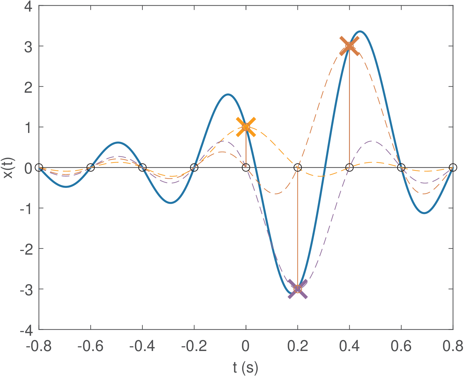
In this example, the first sinc in Figure 1.34 is centered at $t = 0$ (corresponding to $δ [n]$ ). The second and third sincs are $- 3 sinc (\frac{t - 0.2}{0.2})$ and $3 sinc (\frac{t - 0.4}{0.2})$ , respectively. The summation of these three parcels according to Eq. (1.28), results in the analog signal

x (t) = sinc (t ∕ 0.2) - 3 sinc ((t - 0.2) ∕ 0.2) + 3 sinc ((t - 0.4) ∕ 0.2),

(1.29)

which is depicted with a continuous (instead of dashed) line.

The circles in Figure 1.34 indicate the time instants $t = n T_{s}$ and the $\times$ marks indicate the amplitude in the position of each of the three impulses. Note that $x (t)$ has an infinite support (duration) but has zero amplitude at $t = n T_{s}$ , except for $n = 0, 1$ and 2. These are discrete-time values corresponding to the support of $x [n]$ . $□$

1.7.8 Discrete-time to continuous-time (D/C) conversion

The discrete-time to continuous-time (D/C) conversion is the inverse of C/D and can be represented as the following block diagram:

x [n] \to D ∕ S \to x_{s} (t) \to RECONSTRUCTION \to x (t)

that illustrates the D/C conversion is composed by D/S followed by RECONSTRUCTION.

1.7.9 Analog to digital (A/D) and digital to analog (D/A) conversions

The A/D and D/A processes differ from C/D and D/C, respectively, because the former pair incorporates quantization such that the amplitude values can be represented with a finite number of bits and processed or stored in digital hardware. The distinction between D/C and D/A conversions is that the inputs are, respectively, a discrete-time $x [n]$ and a digital signal $x_{q} [n]$ . For instance, the following block diagram illustrate the signals involved in a D/A process: digital $x_{q} [n]$ , quantized-sampled $x_{s, q} (t)$ and analog $x (t)$ :

x_{q} [n] \to D ∕ S \to x_{s, q} (t) \to RECONSTRUCTION \to x (t) .

Example 1.27. Example of a D/A process. Figure 1.35 provides an example of a complete D/A process.

Figure 1.35: Signal reconstruction of a signal with quantized amplitudes using ZOH.

Figure 1.35 illustrates D/A assuming RECONSTRUCTION using ZOH, a digital signal $x_{q} [n]$ with amplitudes from the set $ℳ = {- 3, - 1, 1, 3}$ and $T_{s} = 0.2$ s. $□$

Both Figure 1.35 and Figure 1.32 illustrate ZOH reconstruction, but in Figure 1.35 the amplitudes of $x (t)$ are limited to the given finite set (quantized amplitudes) used in $x_{q} [n]$ .

One could denote the ZOH output in Figure 1.35 as $x_{q} (t)$ to emphasize the amplitude is quantized, but most practical reconstruction schemes (other than ZOH) generate an analog signal with amplitudes not belonging to $ℳ$ and it is more general to denote the output of a reconstruction stage as $x (t)$ instead of $x_{q} (t)$ .

Having all these concepts defined, Figure 1.36 illustrates a complete processing chain of an input analog signal $x (t)$ that generates the output $y (t)$ . The core of the processing is the digital signal processing (DSP) block, which can implement, for instance, a digital filter. Often, the same sampling frequency value $F_{s}$ is used by both A/D and D/A processes.¹² Note that the sampled signals $x_{s} (t)$ and $y_{q, s} (t)$ do not actually exist within ADC or DAC chips, but are useful abstract models for the input of the S/D process and output of the D/S process, respectively.

Figure 1.36: Complete processing chain of an input analog signal $x (t)$ to generate an output $y (t)$ using DSP.

1.7.10 Sampling theorem

The sampling theorem specifies the minimum value that $F_{s}$ must assume in order to be able to perfectly reconstruct $x (t)$ from $x_{s} (t)$ or the respective $x [n]$ . It is stated here without proof, which is deferred to Chapter 3.

Theorem 1. Sampling theorem. Assuming the maximum frequency of a real-valued signal $x (t)$ is $f_{max}$ , the sampling frequency must obey

F_{s} > 2 f_{max},

(1.30)

in order to guarantee the perfect reconstruction of $x (t)$ from its sampled version $x_{s} (t)$ or the corresponding $x [n]$ . If $f_{max}$ is given in Hz, $F_{s}$ is the number of real-valued samples per second, also given in Hz (alternatively, it can be denoted in samples per second, or SPS). $□$

Sampling is so important that it will be further discussed later with the help of Fourier transforms in Section 3.5. But before delving into a more rigorous mathematical description of sampling, it is useful to understand the expression of a periodic impulse train

p (t) = \sum_{k = - \infty}^{\infty} δ (t - k T_{s}),

where $T_{s}$ is the sampling interval and $k \in ℤ$ . The expression for $p (t)$ and the sifting property of the impulse allows to model the sampled signal as

x_{s} (t) = x (t) p (t) = \sum_{k = - \infty}^{\infty} x (k T_{s}) δ (t - k T_{s}) .

(1.31)

The S/D stage can then convert $x_{s} (t)$ into $x [n]$ , which represents $x (t)$ .

In Eq. (1.30), perfect reconstruction means that given the sample values, specified as $x_{s} (t)$ or $x [n]$ , it is possible to recover the original $x (t)$ . But in this case, the reconstruction process is not as simple as the ZOH in Figure 1.35. The ideal (“perfect”) reconstruction adopts the infinite-duration sinc function as discussed in Section 1.7.7.0. More specifically, $x (t)$ is obtained from Eq. (1.28) as the following combination of scaled and shifted versions of $h (t) = sinc (t ∕ T_{s})$ :

x (t) = \sum_{n = - \infty}^{\infty} x [n] sinc (\frac{t - n T_{s}}{T_{s}}) .

(1.32)

A continuous-time signal $x (t)$ with infinite duration often requires an infinite number of samples to be fully represented. This can be seen by sampling an eternal sinusoidal signal according to the sampling theorem. For instance, $x (t) = 3 cos (20 πt)$ has angular frequency $ω = 20 π$ rad/s and frequency 10 Hz. Assuming C/D conversion with $F_{s} = 40$ Hz, leads to $x [n] = \dots + 3 δ [n + 4] - 3 δ [n + 2] + 3 δ [n] - 3 δ [n - 2] + 3 δ [n - 4] - 3 δ [n - 6] + \dots$ , which corresponds to repeating the amplitude values $3, 0, - 3, 0$ from $n = - \infty$ to $\infty$ . Hence, the original signal $x (t)$ can be perfectly reconstructed from $x [n]$ using Eq. (1.32). In this case, the infinite number of sinc parcels in Eq. (1.32) would properly add to perfectly compose the original signal $x (t) = 3 cos (20 πt)$ .

The following example aims at providing a more concrete description of reconstructing a sinusoid. Instead of trying to use an eternal sinusoid and infinite sinc parcels, an approximation is used for a specific time interval.

Example 1.28. Example of cosine reconstruction from few samples. This examples adopts oversampling (see Section 1.7.2) to generate a high-resolution discrete-time signal that resembles the original analog signal. Listing 1.10 describes all preparation steps for invoking the function ak_sinc_reconstruction.m.

Listing 1.10: MatlabOctaveCodeSnippets/snip_signals_cosine_reconstruction.m. [ Python version]

1%% Define variables 
2max_n = 8; %n varies from -max_n to max_n 
3Ts=0.2; %sampling interval (in seconds) 
4A=4; %cosine amplitude, in Volts 
5Fs=1/Ts; %sampling frequency (5 Hz) 
6fc=Fs/4; %cosine frequency (1.25 Hz) 
7oversampling_factor = 200; %oversampling factor 
8textra = 1; %one extra time (1 second) for visualizing sincs 
9%% Generate signal xn sampled at Fs 
10n=-max_n:max_n; %original discrete-time axis as integers 
11t=(-max_n:max_n)*Ts; %original sampled time axis in seconds 
12xn=A*cos(2*pi*fc*t); %cosine sampled at Fs 
13%% Generate oversampled version of xn 
14oversampled_Ts = Ts/oversampling_factor; %new value of Ts 
15oversampled_n = n(1)*oversampling_factor:n(end)*oversampling_factor; 
16oversampled_t = oversampled_n*oversampled_Ts; %time in seconds 
17oversampled_xn=A*cos(2*pi*fc*oversampled_t); %oversampled cosine 
18%% Reconstruct signal from samples stored at xn and compare with 
19%% the "ground truth" oversampled_xn 
20ak_sinc_reconstruction(n,xn,Ts,oversampled_n,oversampled_xn,textra);

The low-resolution signal $x [n]$ , or xn in Listing 1.10, represents a segment with only 17 samples obtained by sampling a segment from $t = - 1.6$ to 1.6 s of the original signal $x (t) = A cos (2 π f_{c} t)$ , with $A = 4$ volts and $f_{c} = 1.25$ Hz. Because $F_{s} = 5$ Hz is larger than $2 f_{c}$ Hz, the sampling theorem is obeyed and a perfect reconstruction is possible.

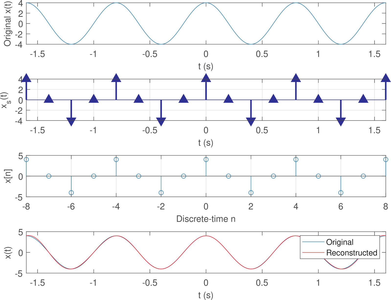
Figure 1.37: Sampling and sinc-based perfect reconstruction of a cosine as implemented in function ak_sinc_reconstruction.m.

The signal oversampled_xn plays the role of the analog signal $x (t)$ within a computer, using a relatively large oversampling factor of 200. This signal is shown in the top plot of Figure 1.37. The second plot from the top is depicting the sampled signal $x_{s} (t)$ , while the third shows the discrete-time signal $x [n] = S/D {x_{s} (t)}$ .

The signal oversampled_xn is passed as an input argument to function ak_sinc_reconstruction.m such that it can be compared to the reconstructed signal created within this function, as depicted in the bottom plot of Figure 1.37. The two plots (“original” and “reconstructed”) overlap almost perfectly. But closely observing the bottom plot in Figure 1.37 shows that the reconstruction is better in the time instants closer to the center $t = 0$ than in the endpoints $t = \pm 1.6$ s. The reason for that can be understood by interpreting Figure 1.38 and Figure 1.39.

Figure 1.38: Single sinc parcel from Figure 1.39 corresponding to the sinc centered at $t = - 0.8$ s as dashed line and the reconstructed signal as a solid line.

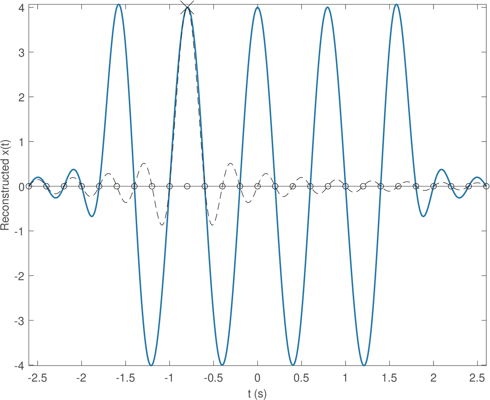
Figure 1.38 depicts a single sinc while Figure 1.39 shows all sinc parcels. Figure 1.38 shows the sinc centered at $t = - 0.8$ s (or $n = - 4$ ) and the reconstructed signal, obtained by using all sinc parcels.

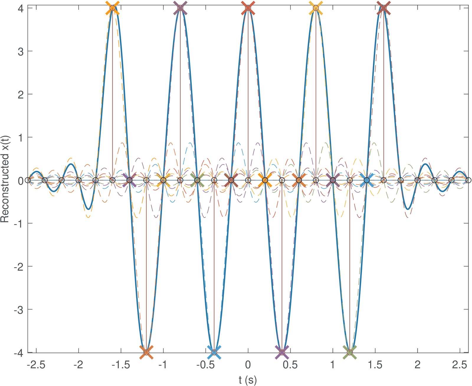
Figure 1.39: All individual parcels in dashed lines corresponding to each sinc and the summation as reconstructed signal (solid line) of Listing 1.10.

Because it has several superimposed curves, the reader is invited to obtain Figure 1.39 by executing ak_sinc_reconstruction.m iteratively, step-by-step, to see each individual sinc being plotted. Figure 1.39 can only depict the final result, with all sincs superimposed. Basically, this figure shows that the scripts was created such that only nine sincs effectively contribute to reconstructing the cosine, given that six samples of $x [n]$ have amplitude equals zero. The reconstruction at the endpoints is impaired because the infinite number of sincs in Eq. (1.32) are not used by the script. The missing sincs at the left ( $t < - 1.6$ ) and right ( $t > 1.6$ ) extrema have more impact at the endpoints than at $t = 0$ . $□$

Example 1.29. Reconstruction of a signal composed by sincs. This example further investigates the reconstruction of the signal described by Eq. (1.29), which is repeated below for convenience:

x (t) = sinc (t ∕ 0.2) - 3 sinc ((t - 0.2) ∕ 0.2) + 3 sinc ((t - 0.4) ∕ 0.2) .

The signal $x (t)$ is composed by three parcels of the sinc

z (t) = sinc (\frac{t}{0.2}) .

Finding the frequencies that compose a signal is the topic of Chapter 2, but it can be anticipated here that the maximum frequency¹³ of $z (t)$ is bounded by $f_{max} < 2.5$ Hz. Shifting $z (t)$ to $t = 0.2$ and $t = 0.4$ , and then adding these three parcels to obtain Eq. (1.29), does not increase the maximum frequency. Hence, the bound $f_{max} < 2.5$ Hz also holds for the signal $x (t)$ .

In the case of $f_{max} < 2.5$ Hz, the sampling theorem states that $F_{s} = 5$ Hz guarantees perfect reconstruction. Listing 1.11 adopted $T_{s} = 0.1$ s, which corresponds to $F_{s} = 1 ∕ T_{s} = 10$ Hz, which also obeys the theorem.

Listing 1.11: MatlabOctaveCodeSnippets/snip_signals_reconstruction_sinc.m. [ Python version]

1%% Define variables 
2Ts=0.1; %sampling interval (in seconds) 
3Fs=1/Ts; %sampling frequency (5 Hz) 
4oversampling_factor = 200; %oversampling factor 
5textra = 0.5; %one extra time (2 seconds) for visualizing sincs 
6sinc_support = 0.2; %support of the sinc in seconds 
7n=-8:12; %segment of samples of interest 
8%% Generate signal xn sampled at Fs 
9t=n*Ts; %discrete-time axis in seconds 
10xn = sinc(t/sinc_support) - 3*sinc((t-0.2)/sinc_support) + ... 
11    3*sinc((t-0.4)/sinc_support); %define the sampled signal 
12%% Generate oversampled version of xn 
13oversampled_Ts = Ts/oversampling_factor; %new value of Ts 
14oversampled_n = n(1)*oversampling_factor:n(end)*oversampling_factor; 
15oversampled_t = oversampled_n*oversampled_Ts; %time in seconds 
16oversampled_xn = sinc(oversampled_t/sinc_support) - ... 
17    3*sinc((oversampled_t-0.2)/sinc_support) + ... 
18    3*sinc((oversampled_t-0.4)/sinc_support); %oversampled signal 
19%% Reconstruct signal from samples stored at xn and compare with 
20%% the "ground truth" oversampled_xn 
21ak_sinc_reconstruction(n,xn,Ts,oversampled_n,oversampled_xn,textra);

Figure 1.40 (bottom plot) illustrates good reconstruction, even when using a segment of limited duration (from $t = - 0.8$ to 1.2 s).

Figure 1.40: Sampling and reconstruction of $x (t) = sinc (t ∕ 0.2) - 3 sinc ((t - 0.2) ∕ 0.2) + 3 sinc ((t - 0.4) ∕ 0.2)$ using $T_{s} = 0.1$ s.

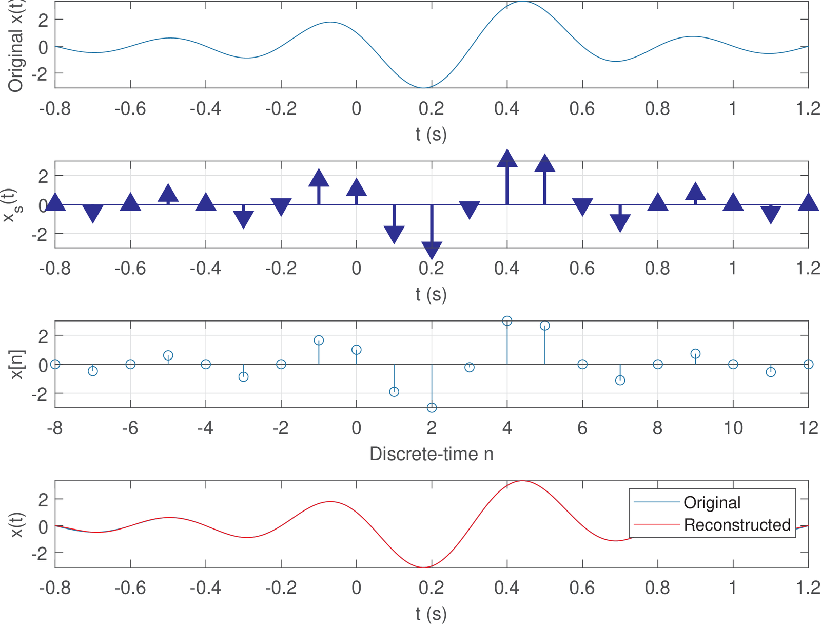
Figure 1.41 is similar to Figure 1.39 and shows the sinc parcels used to reconstruct the signal in Figure 1.40.

Figure 1.41: Sinc parcels used in the reconstruction of $x (t)$ of Figure 1.40.

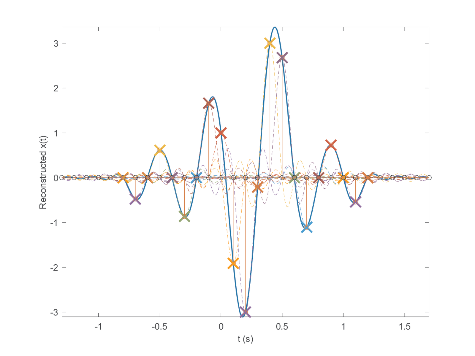
Both Figure 1.40 and Figure 1.33 are derived using the same signal $x (t)$ , but using $T_{s} = 0.1$ and 0.2, respectively. It can be seen from Figure 1.33 that $T_{s} = 0.2$ s has, in this case, the property of representing $x (t)$ with only three non-zero samples. The reason to have only three non-zero samples is that the impulses in the train $p (t) = \sum_{k = - \infty}^{\infty} δ (t - 0.2 k)$ used for sampling, coincide with $x (t)$ having an amplitude of zero, with the exception of $t = 0, 0.2$ and 0.4 seconds, as depicted in Figure 1.34. However, if $T_{s} = 0.1$ s is adopted, an infinite number of samples is required to represent $x (t)$ . $□$

Example 1.30. Failing to reconstruct signals when adopting $F_{s} = 2 f_{max}$ . The sampling theorem is a strict inequality $F_{s} > 2 f_{max}$ but some people state it as a non strict inequality, i. e., $F_{s} \geq 2 f_{max}$ , which is incorrect.

One reason for considering $F_{s} \geq 2 f_{max}$ is wrongly interpreting that $f_{max}$ of the signal described by Eq. (1.29) is $f_{max} = 2.5$ Hz. Because in this case $F_{s} = 5$ Hz works, it may lead to the incorrect assumption that $F_{s} \geq 2 f_{max}$ always works. However, the signal of Eq. (1.29) has infinite frequency components, which extend from zero up to 2.5 Hz, but it does not have a discrete component at $2.5$ Hz. Hence, its $f_{max} < 2.5$ Hz and $F_{s} = 5$ Hz obeys the sampling theorem, and allows perfect reconstruction, as can be seen in Figure 1.33.

However, if a signal has a discrete component at $f_{max}$ , then choosing $F_{s} = 2 f_{max}$ does not guarantee reconstruction. A simple example is to consider sampling the signals $y (t) = cos (2 π \times 2.5 t)$ and $x (t) = cos (2 π \times 2.5 t - 0.5 π)$ using $F_{s} = 5$ Hz. Both signals have $f_{max} = 2.5$ Hz, but the time delay created by the phase $0.5 π$ makes the sampling instants coincide with the zeros of $x (t)$ . In this case, $x_{s} (t)$ (and, consequently $x [n]$ ) has amplitudes equal to zero, and reconstruction fails. This is indicated in Figure 1.42, created with the script snip_signals_failed_cosine_reconstruction.m. This script can be modified to show that $y (t)$ can be eventually reconstructed, but it is not guaranteed. In summary, one must use $F_{s} > 2 f_{max}$ to guarantee perfect reconstruction.

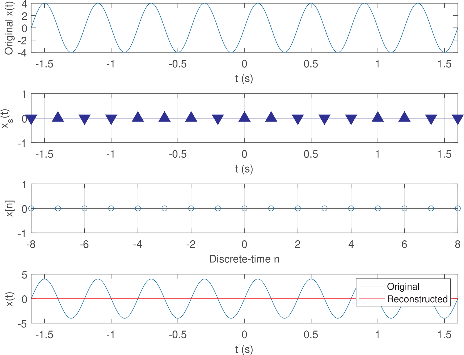
Figure 1.42: Example of failing to reconstruct the signal $x (t) = cos (2 π 2.5 t - 0.5 π)$ using $F_{s} = 2 f_{max} = 5$ Hz.

As another example, assume a cosine

x (t) = A cos (2 π f_{0} t + 𝜃),

(1.33)

where $A = 1 ∕ cos (𝜃)$ . The sampling frequency is (wrongly) chosen as $F_{s} = 2 f_{0}$ such that $x (n) = cos (πn) = {(- 1)}^{n}$ and $x (t)$ cannot be recovered from $x [n]$ (which is the same for any phase $𝜃$ ), as illustrated by Listing 1.12.

Listing 1.12: MatlabOctaveCodeSnippets/snip_signals_sampling_inequality.m. [ Python version]

1Fs=20; Ts=1/Fs; %sampling frequency Fs in Hz and period Ts in sec. 
2f0=Fs/2; %key thing: Fs should  be greater than 2 f0 
3t=0:Ts:1; %discrete-time axis, from 0 to 1 second 
4theta1=pi/4 %define an arbitrary angle 
5A1=1/cos(theta1); %amplitude 
6x1=A1*cos(2*pi*f0*t+theta1); %not obeying sampling theorem 
7theta2=0 %define any value distinct from theta1 
8A2=1/cos(theta2); %amplitude 
9x2=A2*cos(2*pi*f0*t+theta2); %not obeying sampling theorem 
10plot(t,x1,'rx',t,x2,'o-b'); title('Cannot distinguish 2 signals!')

This ambiguity and the previous example demonstrate the need for a strict inequality $F_{s} > 2 f_{max}$ when interpreting the sampling theorem. $□$

Example 1.31. Trying to prove that the sampling theorem is wrong! A very astute student compared Figure 1.11 and Figure 1.33, and observed that two distinct signals could have generated the samples in $x [n] = δ [n] - 3 δ [n - 1] + 3 δ [n - 2]$ . Hence, she concluded that the sampling theorem was wrong, given that from the samples $x [n]$ , one would not be able to distinguish if the original signal corresponds to Eq. (1.7) or Eq. (1.29).

Her main mistake was not to check the maximum frequencies of the signals given by Eq. (1.7) or Eq. (1.29). Finding the frequencies that compose a signal is the topic of Chapter 2, but it can be anticipated here that the maximum frequency of Eq. (1.29) is $f_{max} = 2.5$ Hz (from Eq. (A.56)) while the signal corresponding to Eq. (1.7) has an infinite maximum frequency (from Eq. (A.54)) and its conversion to $x [n]$ did not obey the sampling theorem!

Listing 1.13 illustrates what happens when one starts with Eq. (1.7), samples this signal (but not obeying the sampling theorem) and then tries to recover Eq. (1.7) using sinc interpolation. The generated Figure 1.43 shows that reconstruction fails miserably.

Listing 1.13: MatlabOctaveCodeSnippets/snip_signals_reconstruction_failure.m. [ Python version]

1%% Define variables 
2Ts=0.2; %sampling interval (in seconds) 
3Fs=1/Ts; %sampling frequency (5 Hz) 
4oversampling_factor = 200; %oversampling factor 
5textra = 1; %one extra time (1 second) for visualizing sincs 
6pulse_width = 0.2; %support of the rects in seconds 
7%% Generate signal xn sampled at Fs 
8n=-3:3; 
9xn=[0 0 0 1 -3 3 0]; %signal with only three non-zero samples 
10%% Generate oversampled version of xn 
11oversampled_Ts = Ts/oversampling_factor; %new value of Ts 
12oversampled_n = n(1)*oversampling_factor:n(end)*oversampling_factor; 
13oversampled_t = oversampled_n*oversampled_Ts; %time in seconds 
14oversampled_xn = rectpuls(oversampled_t,pulse_width) - ... 
15    3*rectpuls(oversampled_t-Ts,pulse_width) + ... 
16    3*rectpuls(oversampled_t-2*Ts,pulse_width); %define the signal 
17%% Reconstruct signal from samples stored at xn and compare with 
18%% the "ground truth" oversampled_xn 
19ak_sinc_reconstruction(n,xn,Ts,oversampled_n,oversampled_xn,textra);

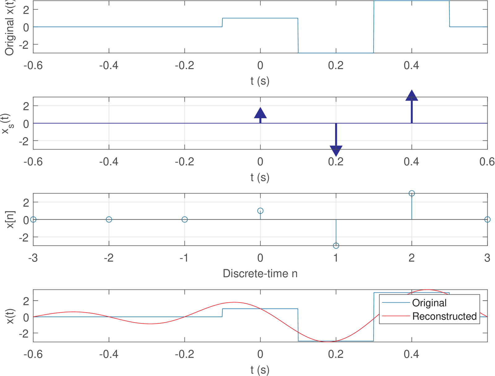
Figure 1.43: Reconstruction of signal given by Eq. (1.7) fails because the sampling theorem is not obeyed.

Figure 1.44 is similar to Figure 1.39 and shows the sinc parcels used to reconstruct the signal.

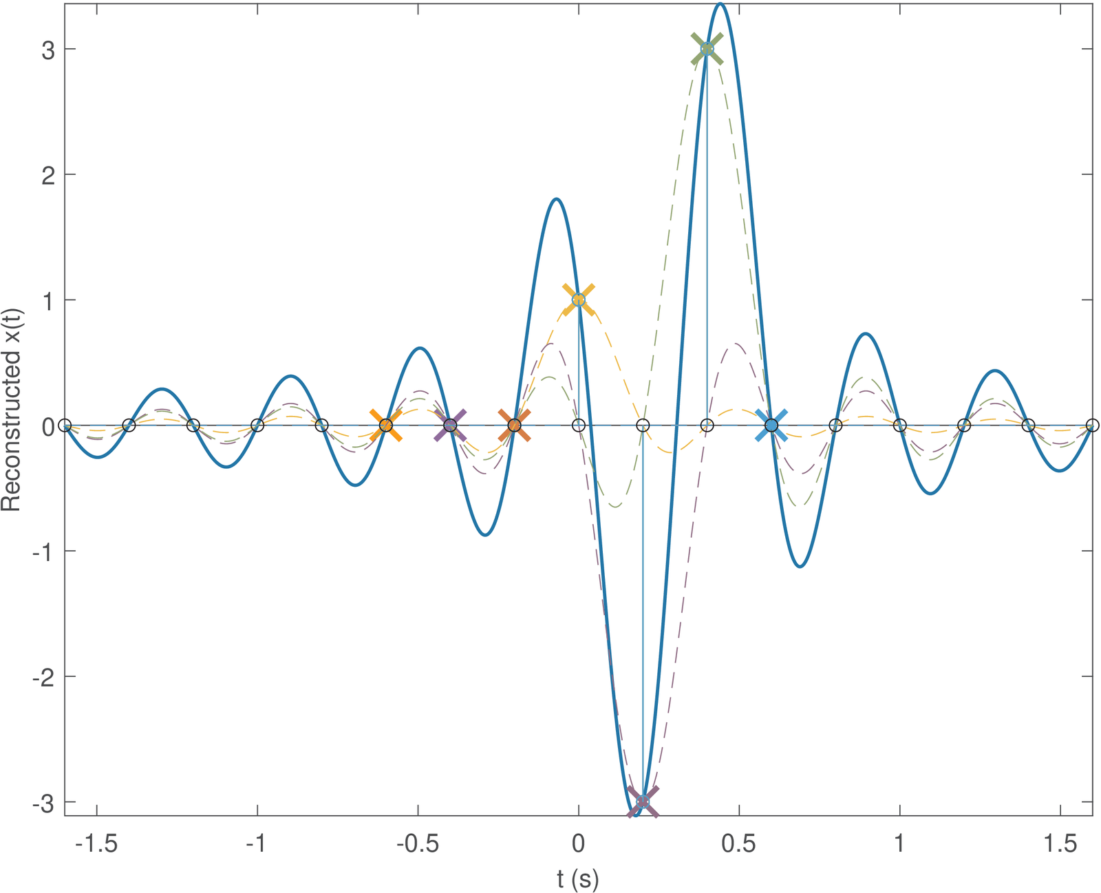
Figure 1.44: Sinc parcels used in the signal reconstructed as depicted in Figure 1.43.

The main message of this example is the proper interpretation of the sampling theorem: there is a unique continuous-time signal that has $f_{max} < F_{s} ∕ 2$ and is represented by a given sampled signal $x_{s} (t)$ , or equivalently, $x [n]$ . In this specific case, Eq. (1.29) is the only signal $x (t)$ that can lead to $x [n] = δ [n] - 3 δ [n - 1] + 3 δ [n - 2]$ . $□$

The perfect reconstruction guaranteed by the sampling theorem, Eq. (1.30), assumes the use of the ideal sinc interpolation of Eq. (1.32), which is not realizable in practice. Hence, $F_{s}$ is chosen to be typically $2.5 f_{max}$ or even larger to alleviate the errors imposed by a non ideal reconstruction. The sampling frequencies adopted for some common signals¹⁴ are shown in Table 1.4.

Table 1.4: Typical sampling frequencies.

Signal	$f_{max}$	Explanation for $f_{max}$	$F_{s}$
Telephone speech	3400 Hz	Band [300, 3400] Hz suffices for intelligibility	8 kHz
Audio (CD format)	20 kHz	Humans can hear up to $\sim$ 20 kHz	44.1 kHz
Electrocardiogram (ECG)	$< 250$ Hz	Clinical studies	500 Hz

In special cases, when $x (t)$ is complex-valued or a “passband” signal (Section 3.5.5), a lower value of $F_{s}$ can be adopted and still allow perfect reconstruction.

1.7.11 Different notations for S/D conversion

It is convenient to have two different notations for the S/D conversion: a simpler one and an alternative that better represents cases in which the amplitude of $x [n]$ depends on the sampling interval $T_{s}$ . We start this discussion with an example.

Example 1.32. Example of S/D conversion of a signal $x_{s} (t)$ . Assume the continuous-time signal $x (t) = 4 e^{- 2 t} u (t)$ should be sampled with a period $T_{s}$ to create $x_{s} (t)$ , which is then transformed into a discrete-time signal $x [n]$ via the S/D operation. The notation $S/D {\cdot}$ will denote the S/D process, which in this case leads to:

\begin{array}{l} x [n] & = S/D {x_{s} (t)} \\ = S/D {\sum_{n = - \infty}^{\infty} x (n T_{s}) δ (t - n T_{s})} \\ = S/D {\sum_{n = - \infty}^{\infty} 4 e^{- 2 n T_{s}} u (n T_{s}) δ (t - n T_{s})} \\ = 4 e^{- 2 n T_{s}} u [n], & (1.34) \end{array}

The last step in Eq. (1.34) is based on the fact that $S/D {u (n T_{s}) δ (t - n T_{s})} = u [n]$ . $□$

When writing signal expressions, the sampling operation is eventually not made explicit. An alternative notation is discussed in the following example.

Example 1.33. Simplified notation for the S/D conversion of a signal $x (t)$ . This example discusses a simplified notation for the S/D conversion that is sometimes adopted in the literature.

Assume the continuous-time signal $x (t) = 4 e^{- 2 t} u (t)$ should be transformed to a discrete-time $x [n]$ with a sampling period $T_{s}$ . This conversion is often denoted as:

x [n] = x (t) |_{t = n T_{s}} = 4 e^{- 2 n T_{s}} u [n],

(1.35)

which can be confusing. One could write $x (t) |_{t = n T_{s}} = 4 e^{- 2 n T_{s}} u (n T_{s})$ and, comparing to Eq. (1.35), complain that the samples of the continuous-time step function $u (n T_{s})$ became $u [n]$ ( $n T_{s}$ was “substituted” by $n$ ), while $n T_{s}$ remained (was not substituted by $n$ ) in the exponential $e^{- 2 n T_{s}}$ .

The reason to be careful with the simplified notation $x [n] = x (t) |_{t = n T_{s}}$ is that, when performing a S/D conversion, the occurrences of $n T_{s}$ as part of the independent variable (the argument $t$ of $x (t)$ , within $(⋅)$ ) are converted to $n$ , as depicted in Figure 1.30. However, the factor $n T_{s}$ remains when it influences the amplitude (dependent variable).

Hence, the notation $x [n] = x (t) |_{t = n T_{s}}$ for the S/D process in Eq. (1.35) is somehow incomplete. It does not rely on impulses and, consequently, it does not make explicit the intermediate step of creating a sampled signal $x_{s} (t)$ . However, because the $S/D {\cdot}$ notation is cumbersome, the reader should be also familiar with the widely adopted alternative of Eq. (1.35). $□$

¹¹ Eq. (1.27) represents the convolution between $x_{s} (t)$ and $h (t)$ . Convolution will be discussed in Section 3.4.1 and allows $h (t)$ to be interpreted as the impulse response of a filter used for reconstruction.

¹² But in general, multiple sampling frequencies can be adopted at distinct stages of a signal processing chain. In this case, one can use multirate signal processing.

¹³ This $f_{max}$ value is obtained from Eq. (A.56) with $F = 2.5$ Hz, and observing that the spectrum of $x (t)$ extends up to 2.5 Hz but does not have an impulse at this frequency, indicating that there is no frequency component at 2.5 Hz, and $f_{max} < 2.5$ Hz.

¹⁴ ECG is discussed, for example, at [ url1ecg].