1.10  Correlation: Finding Trends

It is often useful to infer whether or not random variables are related to each other via correlation. For example, height and weight are quantities that present positive correlation for the human population. However, happiness and height are uncorrelated. There are measures other than correlation to detect similarities among variables, such as the mutual information, but correlation is simple and yet very useful. Correlation is called a second-order statistics because it considers only pairwise or quadratic dependence. It does not detect non-linear relations nor causation, that is, correlation cannot deduce cause-and-effect relationships. But correlation helps to indicate trends such as one quantity increasing when another one decreases.

The correlation $C$ for two complex-valued random variables $X$ and $Y$ is defined as

where $\ast$ denotes the complex conjugate. The correlation coefficient, which is a normalized version of the covariance (not correlation), is defined as

where the covariance is given by

Note that, when one wants to fully identify the statistical moments of two complex random variables, it is convenient to separately identify the interactions among their real and imaginary parts and organize the partial results of Eq. (1.47) as a $2\times 2$ matrix. Real-valued random variables are assumed hereafter. When the random variables are real-valued, Eq. (1.47) simplifies to

Two real-valued random variables are called uncorrelated if, and only if, $\mathrm{\text{cov}}(X,Y)=0$, which is equivalent to

As mentioned, $\rho$ is calculated by extracting the means $𝔼[X]={\mu }_x$ and $𝔼[Y]={\mu }_y$, i. e., using $\mathrm{\text{cov}}(X,Y)$ instead of $\mathrm{\text{cor}}(X,Y)$, and is restricted to $-1\le \rho \le 1$ when the random variables are real-valued. Application 1.9 gives an example of using correlation to perform a simple data mining.

1.10.1  Autocorrelation function

Autocorrelation functions are extension of the correlation concept to signals. Table 1.9 summarizes the definitions that will be explored in this text.

The existence of distinct autocorrelation definitions for power and energy signals illustrate the importance of distinguishing them, as discussed in Section 1.6.4.

Advanced: Definitions of autocorrelation for random signals

An autocorrelation function (ACF) defined for stochastic processes (see Appendix A.20) is

which corresponds to the correlation between random variables $X(s)$ and $X(t)$ at two different points $s$ and $t$ in time of the same random process where $X^{\ast }(t)$ is the complex conjugate of $X(t)$. The purpose of the ACF is to determine the strength of relationship between amplitudes of the signal occurring at two different time instants.

For wide-sense stationary (WSS) processes, the ACF is given by

where the time difference $\tau =s-t$ is called the lag time.

The random process formalism is very powerful and allows for representing complicated processes. But in many practical cases only one realization $x(t)$ (or $x[n]$) of the random process $X(t)$ is available. The alternative to deal with the signal without departing from the random process formalism is to assume that $X(t)$ is ergodic. In this case, the statistical (or ensemble) average represented by $𝔼[\cdot ]$ is substituted by averages over time.

The definitions of autocorrelation given by Eq. (1.49) and Eq. (1.50) are the most common in signal processing, but others are adopted in fields such as statistics. Choosing one depends on the application and the model adopted for the signals.

When dealing with a simple signal, one can naturally adopt one of the definition of autocorrelation for deterministic signals discussed in the sequel.

Definitions of autocorrelation for deterministic signals

A definition of ACF tailored to a deterministic (non-random) energy signal $x(t)$, which does not use expected values as Eq. (1.49), is

such that

where $E$ is the signal energy. It should be noted that this definition of autocorrelation cannot be used for power signals. Power signals have infinite energy and using Eq. (1.51) for $\tau =0$ leads to $R_X(0)=\infty$ in the case of power signals, which is uninformative.

If $x(t)$ is a deterministic power signal, an useful ACF definition is

such that

where $P$ is the signal average power. Eq. (1.53) can also be used when $x(t)$ is a realization of an ergodic stochastic process.

Similarly, there are distinct definitions of autocorrelation for deterministic discrete-time signals. For example, when $x[n]$ is a finite-duration real signal with $N$ samples, the (unscaled or not normalized) autocorrelation can be written as

which has a minus in $n-i$ that does not lead to reflecting the signal.¹⁷

As an alternative to use expressions more similar to the ones for signals with infinite duration, the (unscaled or not normalized) autocorrelation can be expressed as

and computed assuming a zero value for $x[n]$ when its index is out of range. This corresponds to assuming the signal is extended with enough zeros (zero-padding) to the right and to the left. For example, assuming $x[n]=\delta [n]+2\delta [n-1]+3\delta [n-2]$, which can be represented by the vector $[1,2,3]$, its autocorrelation would be $[3,8,14,8,3]$, for the lags $i=-2,-1,0,1,2$, respectively.

Note in Table 1.10 that the number of products decreases as $|i|$ increases. More specifically, when computing $R_X[i]$ there are only $N-|i|$ “valid” products. To cope with that, the normalized (and statistically unbiased) definition is

In Matlab/Octave, the unbiased estimate for the signal $[1,2,3]$ can be obtained with:

1x=[1,2,3];xcorr(x,'unbiased')

which outputs [3,4,4.67,4,3]. The unscaled estimate of Table 1.10 can be obtained with xcorr(x,’none’) or simply xcorr(x) because it is the default.

Another observation of interest is that for real signals, $R_X(\tau )=R_X(-\tau )$. In general, for complex-valued signals, $R_X(\tau )=R_X^{\ast }(-\tau )$, which is called Hermitian symmetry. Table 1.11 provides an example. It can also be noted that, for a given lag $i$, the subtraction of the indexes of all parcels in valid products is $(n+i)-n=i$.

Example 1.49. Software implementation of autocorrelation. The definitions of $R_X[i]$ used a generic summation ${\sum <!--\; FUNCTION\; APPLICATION\; -->}_n$ over $n$. To be more concrete, an example of Matlab/Octave code to calculate the unscaled autocorrelation $R_X[i]$ is given in Listing 1.20. It can be seen that the property $R_X(\tau )=R_X^{\ast }(-\tau )$ is used to obtain the autocorrelation values for negative $\tau$.

1%Calculate the unscaled autocorrelation R(i) of x 
2x=[1+j 2 3] %define some vector x to test the code 
3N=length(x); 
4R=zeros(1,N); %space for i=0,1,...N-1 
5R(1)=sum(abs(x).^2); %R(0) is the energy 
6for i=1:N-1 %for each positive lag 
7    temp = 0; %partial value of R 
8    for n=1:N-i %vary n over valid products 
9        temp = temp + x(n+i)*conj(x(n)); 
10    end 
11    R(i+1)=temp; %store final value of R 
12end 
13R = [conj(fliplr(R(2:end)))] %append complex conjugate
  

The function xcorr in Matlab/Octave uses a much faster implementation based on the fast Fourier transform (FFT), to be discussed in Chapter 2. When comparing the results of the two methods, the discrepancy is around $10^{-14}$, which is a typical order of magnitude for numerical errors when working with Matlab/Octave.    $\text{□}$

When infinite duration power signals can be assumed, it is sensible to define

Examples of some signals autocorrelations

Two examples of autocorrelation are discussed in the sequel.

Example 1.50. Autocorrelation of white signal. A signal is called “white” when it has an autocorrelation $R[i]=\mathit{A\delta }[i]$ in discrete-time, or $R(\tau )=\mathit{A\delta }(\tau )$ in continuous-time, where $A\in ℝ$ is an arbitrary value. In other words, a white signal has an autocorrelation that is nonzero only at the origin, which corresponds to having samples that are uncorrelated and, consequently, statistically independent.

This nomenclature will be clarified in Chapter 4 but it can be anticipated that such signals have their power uniformly distributed over frequency and the name is inspired by the property of white light, which is composed by a mixture of color wavelengths.

As mentioned, the samples of a white signal are independent and, if they are also identically distributed according to a Gaussian PDF, the signal is called white Gaussian noise (WGN). More strictly, a WGN signal can be modeled as a realization of a wide-sense stationary process. In this case, WGN denotes the stochastic process itself. Using Matlab/Octave, a discrete-time realization of WGN can be obtained with function randn, as illustrated in Section 1.6.2.    $\text{□}$

Example 1.51. Autocorrelation of sinusoid. Using Eq. (1.53), the autocorrelation of a sinusoid $x(t)=A\text{sin}<!--\; FUNCTION\; APPLICATION\; -->(\mathit{\omega t}+\varphi )$ can be calculated as follows:

We now assume $a=\mathit{\omega t}+\varphi$ for simplicity and use Eq. (A.4) to expand $\text{sin}<!--\; FUNCTION\; APPLICATION\; -->(\mathit{\omega t}+\varphi +\mathit{\omega \tau })$:

The third equality used Eq. (A.9) and Eq. (A.5), and it was simplified because the integrals of both $\text{cos}<!--\; FUNCTION\; APPLICATION\; -->(2a)$ and $\text{sin}<!--\; FUNCTION\; APPLICATION\; -->(2a)$ are zero given the integration interval is an integer number of their periods. The final result indicates that the autocorrelation of a sinusoid or cosine does not depend on the phase $\varphi$ and is also periodic in $\tau$, with the same period $2\pi ∕\omega$ that the sinusoid has in $t$. Therefore, the frequencies contained in the realizations of a stationary random process can be investigated via the autocorrelation $R(\tau )$ of this process.

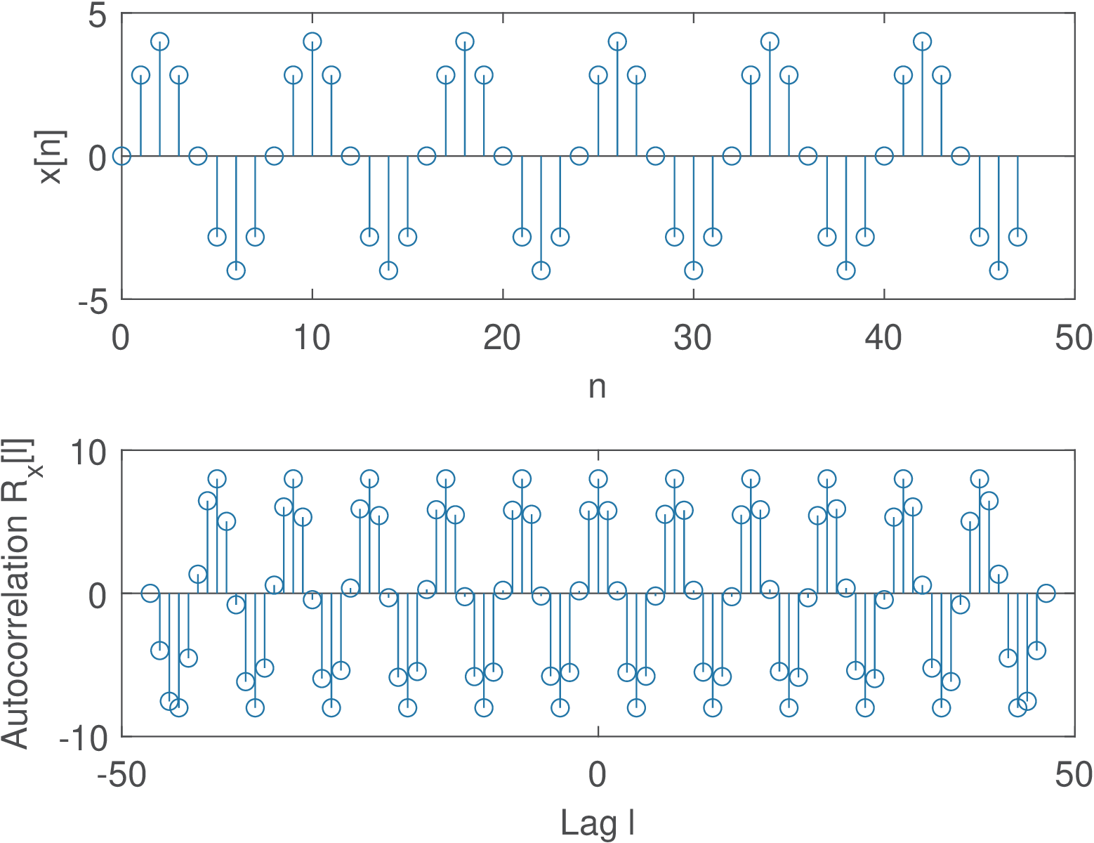
A simulation with Matlab/Octave can help understanding this result. Figure 1.54 was generated with Listing 1.21.

1numSamples = 48; %number of samples 
2n=0:numSamples-1; %indices 
3N = 8; %sinusoid period 
4x=4*sin(2*pi/N*n); %sinusoid (try varying the phase!) 
5[R,l]=xcorr(x,'unbiased'); %calculate autocorrelation 
6subplot(211); stem(n,x); xlabel('n');ylabel('x[n]'); 
7subplot(212); stem(l,R); xlabel('Lag l');ylabel('R_x[l]');
  

It can be seen that the x and R are a sine and cosine, respectively, of the same frequency in their corresponding domains (n and l, respectively).

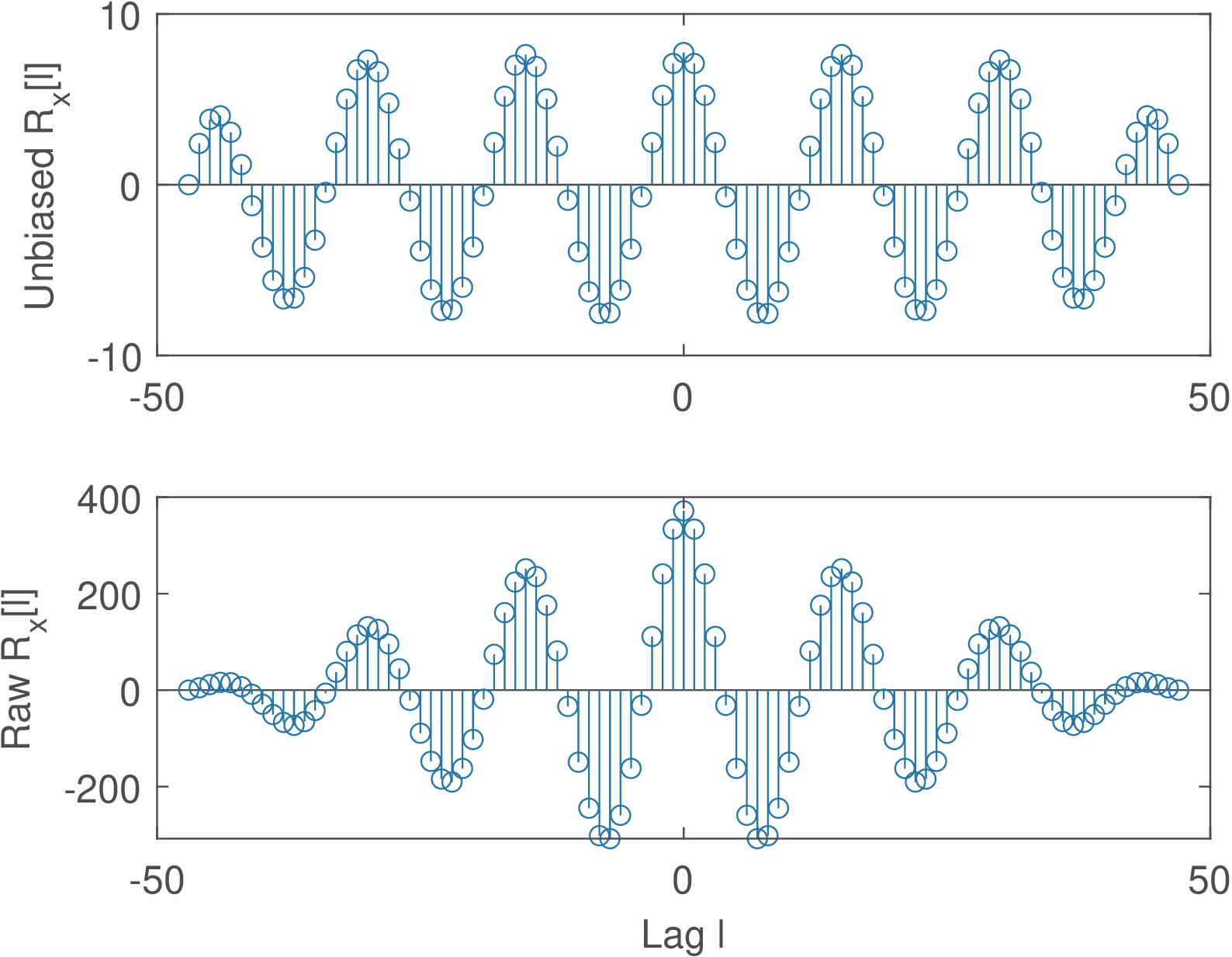
Figure 1.55 was obtained by changing the sinusoid period from N=8 to N=15 and illustrates the effects of dealing with finite-duration signals. Note that both the unbiased and unscaled versions have diminishing values at the end points.    $\text{□}$

Using Eq. (1.57) and a calculation similar to the one used in Eq. (1.58), one can prove that the autocorrelation of $x[n]=\text{sin}<!--\; FUNCTION\; APPLICATION\; -->(\mathrm{\Omega }n+\varphi )$ is $R_X[i]=\text{cos}<!--\; FUNCTION\; APPLICATION\; -->(\mathrm{\Omega }i)∕2$.

1.10.2  Cross-correlation

The cross-correlation function (also called correlation) is very similar to the ACF but uses two distinct signals, being defined for deterministic energy signals as

Note the adopted convention with respect to the complex conjugate.

In discrete-time, the deterministic cross-correlation for energy signals is

Application 1.13 illustrates the use of cross-correlation to align two signals.

Before concluding this section, it is convenient to recall that the autocorrelation of a signal inherits any periodicity that is present in the signal. Sometimes this periodicity is more evident in the autocorrelation than in the signal waveform. The next example illustrates this point by discussing the autocorrelation of a sinusoid immersed in noise.

Example 1.52. The power of a sum of signals is the sum of their powers in case they are uncorrelated. Assume that a sinusoid $x[n]$ is contaminated by noise $z[n]$ such that the noisy version of the signal is $y[n]=x[n]+z[n]$. The signal $z[n]$ is a WGN (see Section 1.10.1.0) that is added to the signal of interest $x[n]$ and, therefore, called additive white Gaussian noise (AWGN). If $x[n]$ and $z[n]$ are uncorrelated, such that $R_{\mathit{xz}}[l]=𝔼[x[n+l]z[n]]=0,\forall <!--\; FUNCTION\; APPLICATION\; -->l$, the autocorrelation $R_y[l]$ of $y[n]$ is given by

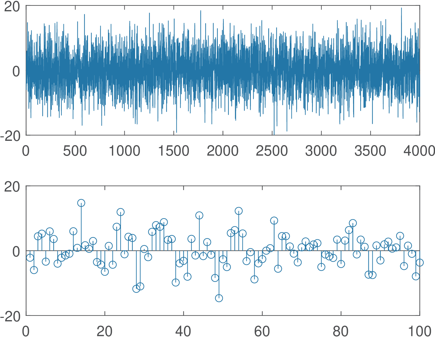
Listing 1.22 illustrates a practical use of this result. A sine with amplitude 4 V and power $4^2∕2=8$ W is contaminated by AWGN with power of 25 W. All signals are represented by 4,000 samples, such that the estimates are relatively accurate.

1%Example of sinusoid plus noise 
2A=4; %sinusoid amplitude 
3noisePower=25; %noise power 
4f=2; %frequency in Hz 
5n=0:3999; %"time", using many samples to get good estimate 
6Fs=20; %sampling frequency in Hz 
7x=A*sin(2*pi*f/Fs*n); %generate discrete-time sine 
8randn('state', 0); %Set randn to its default initial state 
9z=sqrt(noisePower)*randn(size(x)); %generate noise 
10clf, subplot(211), plot(x+z); %plot noise 
11maxSample=100; %determine the zoom range 
12subplot(212),stem(x(1:maxSample)+z(1:maxSample)),pause; %zoom 
13maxLags = 20; %maximum lag for xcorr calculation 
14[Rx,lags]=xcorr(x,maxLags,'unbiased'); %signal only 
15[Rz,lags]=xcorr(z,maxLags,'unbiased'); %noise only 
16[Ry,lags]=xcorr(x+z,maxLags,'unbiased');%noisy signal 
17subplot(311), stem(lags,Rx); ylabel('R_x[l]'); 
18subplot(312),stem(lags,Rz);ylabel('R_z[l]'); 
19subplot(313),stem(lags,Ry);xlabel('Lag l');ylabel('R_y[l]');
  

The signal-to-noise ratio (SNR) is a common metric consisting of the ratio between the signal and noise power values and often denoted in dB (seem Appendix A.24). Figure 1.56 illustrates the fact that it is hard to visualize the sinusoid because of the relatively low signal-to-noise ratio ${\mathrm{\text{SNR}}}_{\mathrm{\text{dB}}}=10{\text{log}<!--\; FUNCTION\; APPLICATION\; -->}_{10}(8∕25)\approx -5$ dB. The waveform does not seem to indicate periodicity.

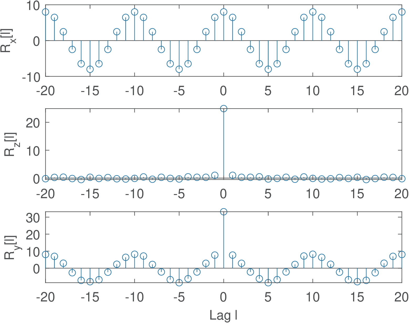
Figure 1.57 shows the autocorrelations of $y[n]$ and its two parcels. For the lag $l=0$, the estimated values are $R_x[0]=8$, $R_z[0]=24.92$ and $R_y[0]=33.17$. The theoretical values are 8 W (the sine power), 25 W (noise power) and $8+25=33$ W (sum of the parcels), respectively. The bottom graph clearly exhibits periodicity and the noise disturbs only the value of $R_y[l]$ at $l=0$. In summary, two assumptions can simplify the analysis of random signals: that the ACF of the noise is approximately an impulse at the origin ($l=0$) and that the signal and noise are uncorrelated.  $\text{□}$

Advanced: Random processes cross-correlation and properties

Some important properties of the cross-correlation are:

• $R_{\mathit{xy}}(\tau )=R_{\mathit{xy}}^{\ast }(-\tau )$ (Hermitian symmetry),
• $R_{\mathit{xy}}(\tau )=R_{\mathit{yx}}^{\ast }(-\tau )$ (swapping arguments is also Hermitian),
• $|R_{\mathit{xy}}(\tau )|\le \sqrt{R_{\mathit{xx}}(0)R_{\mathit{yy}}(0)}$, (maximum is not necessarily at $\tau =0$ but is bounded).

When considering random processes, the two random variables are obtained from distinct processes:

or, assuming stationarity (see Section A.20.0.0) with $s=t+\tau$:

Example 1.53. The AWGN channel. Thermal noise is ubiquitous and WGN is a random process model often present in telecommunications and signal processing applications. WGN was briefly introduced in Examples 1.50, 1.52 and Application 1.10. In telecommunications, distinct systems that share the property of having WGN added at the receiver are called AWGN channel models.

Figure 1.58 illustrates a continuous-time AWGN, where the received signal $r(t)=s(t)+\nu (t)$ is simply the sum of the transmitted signal $s(t)$ and WGN $\nu (t)$.

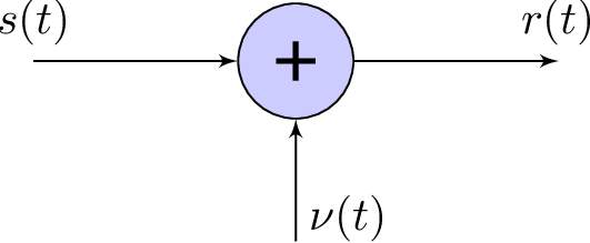
Because $s(t)$ and WGN $\nu (t)$ are often assumed to be uncorrelated, as discussed in Example 1.52, the power of $r(t)$ is the sum of the powers of $s(t)$ and $\nu (t)$.    $\text{□}$

Having learned about correlation (cross-correlation, etc.), it is possible to study a linear model for quantization, which circumvents dealing with the quantizer non-linearity.