Stochastic Processes

A.20 Stochastic Processes

Stochastic or random processes are a powerful formalism for studying signals that incorporate some randomness. While the outcome of a random variable is a number, the outcome of a stochastic process is a time-series, each one called a realization. Hence, when using stochastic processes, it is possible to calculate “time” statistics of a single realization. Besides, one can choose a given time instant and calculate “ensemble” statistics over all realizations at that specific time. These two options may be confusing at first, but are essential. To get intuition on them, the reader is invited to observe the following simple example.

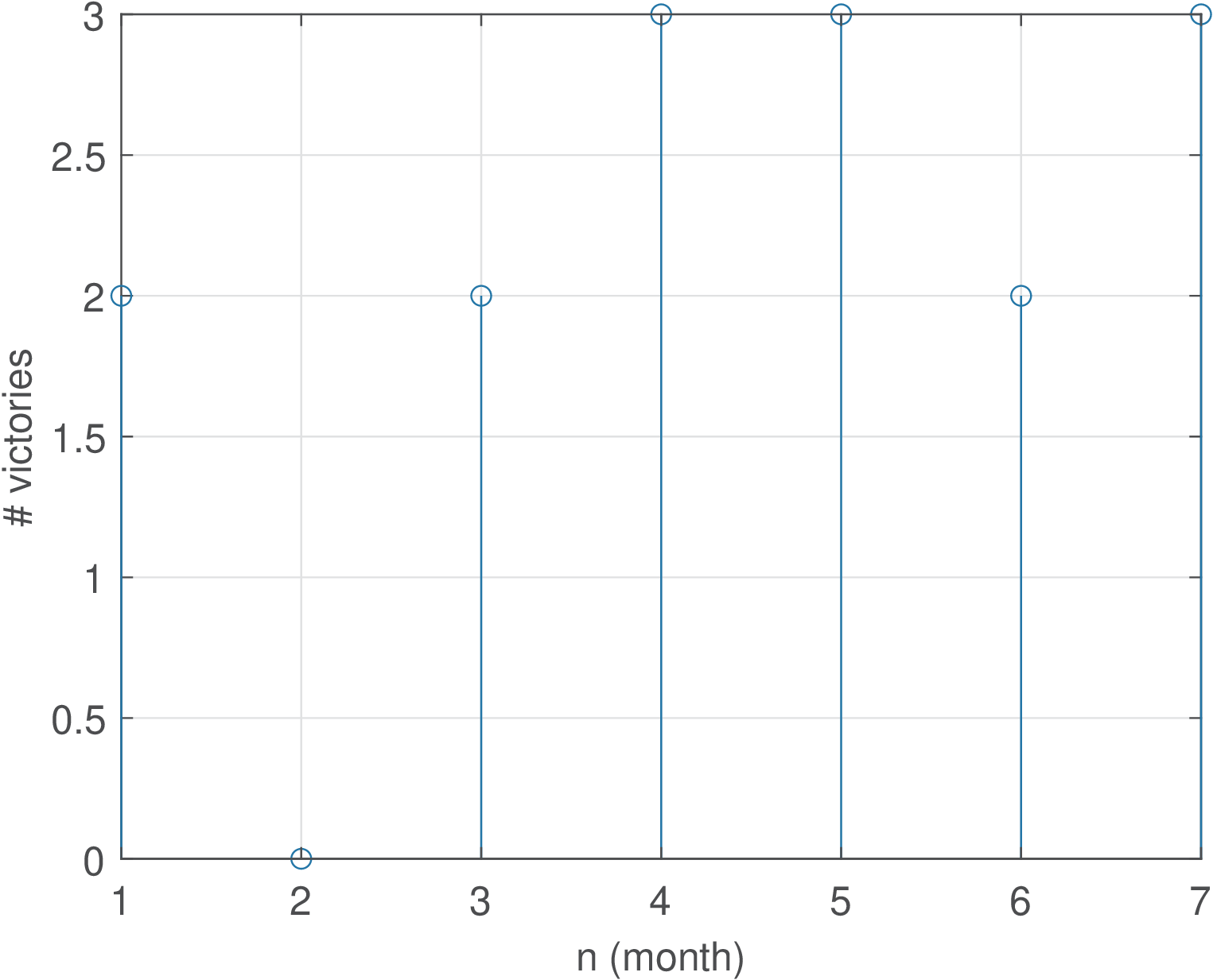
Example A.2. Simple example to explain time and ensemble averages in a stochastic process. Assume a vector [2, 0, 2, 3, 3, 2, 3] where each element represents the outcome of a random variable $X$ indicating the number of victories of a football team in four matches (one per week), along a seven-months season (for example, the team won 2 games in the first month and none in the second). One can calculate the average number of victories as $𝔼 [X] \approx 2.14$ , the standard deviation $σ \approx 1.07$ and other moments of a random variable. This vector could be modeled as a finite-duration random signal $x [n]$ , with Figure A.9 depicting its graph.

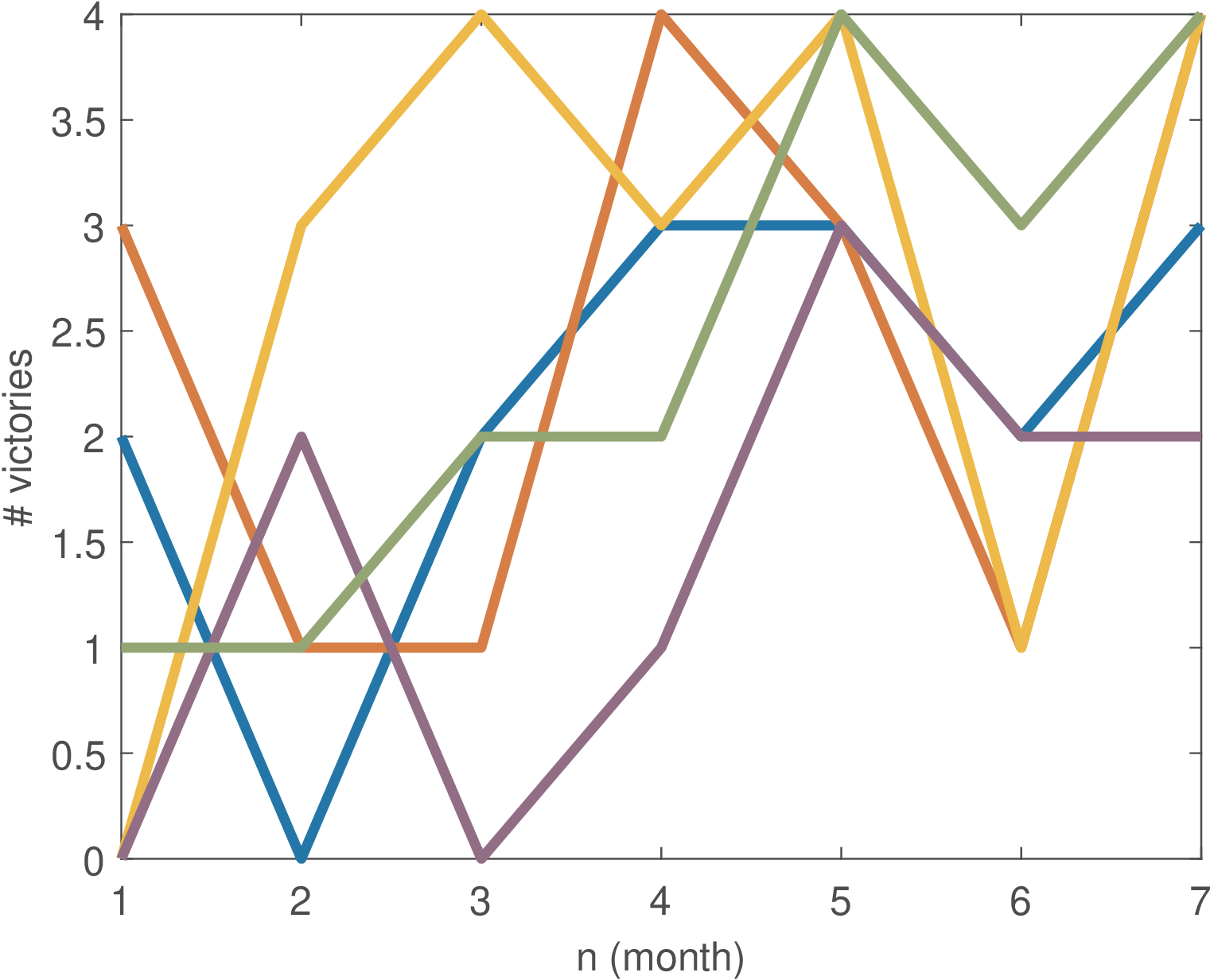
Figure A.9: Example of a finite-duration random signal.

Assume now there are 5 vectors, one for each year. A discrete-time random process can be used to model the data, with each vector (a time series) corresponding to a realization of the random process. For example, following the Matlab convention of organizing different time series in columns (instead of rows), the tabular data below represents the five random signals:

victories = [
     2     3     0     0     1
     0     1     3     2     1
     2     1     4     0     2
     3     4     3     1     2
     3     3     4     3     4
     2     1     1     2     3
     3     4     4     2     4]

Each random signal (column) can be modeled as a realization of a random process. Figure A.10 shows a graphical representation of the data with the five realizations of the example. One should keep in mind that a random process is a model for generating an infinite number of realizations but only 5 are used here for simplicity.

Figure A.10: Example of five realizations of a discrete-time random process.

A discrete-time random process will be denoted by $X [n]$ and one of its realization as $x [n]$ . For the sake of explaining this example, let us define the notation $x_{i} [n]$ to indicate the $i$ -th realization of $X [n]$ . Because $x_{i} [n]$ is a random signal, one can calculate for the given example, $𝔼 [x_{1} [n]] \approx 2.14$ and other statistics taken over time. But a random process is a richer model than a random signal and other statistics can be calculated or, equivalently, more questions can be asked.

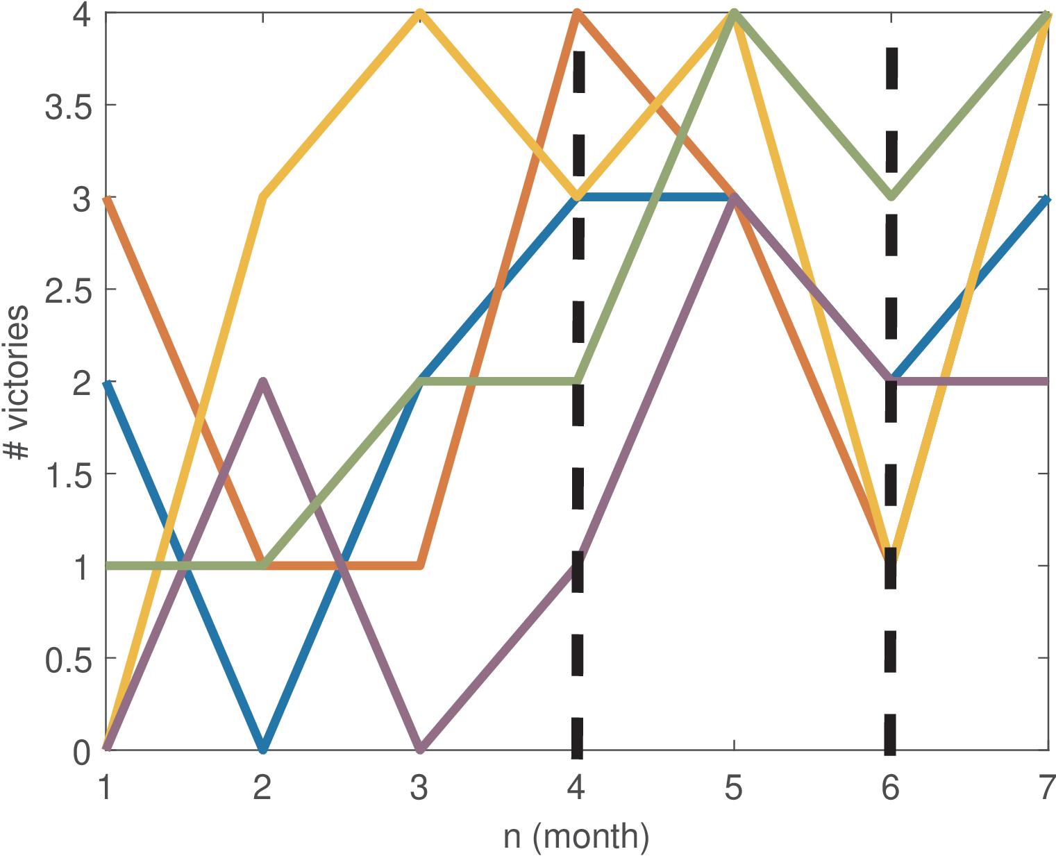
Besides asking for statistics of one realization taken over “time”, it is important to understand that when fixing a given time instant $n_{0}$ , the values that the realizations assume are also outcomes of a random variable that can be denoted by $X [n_{0}]$ . In the example, assuming $n_{0} = 4$ (i.e., assume the fourth month), one can estimate the average $𝔼 [X [4]] = 2.6$ . Similarly, $𝔼 [X [6]] = 1.8$ . Figure A.11 graphically illustrates the operation of evaluating a random process at these two time instants. Differently than the previous time averages, these “ensemble” statistics are obtained across realizations with fixed time instants.

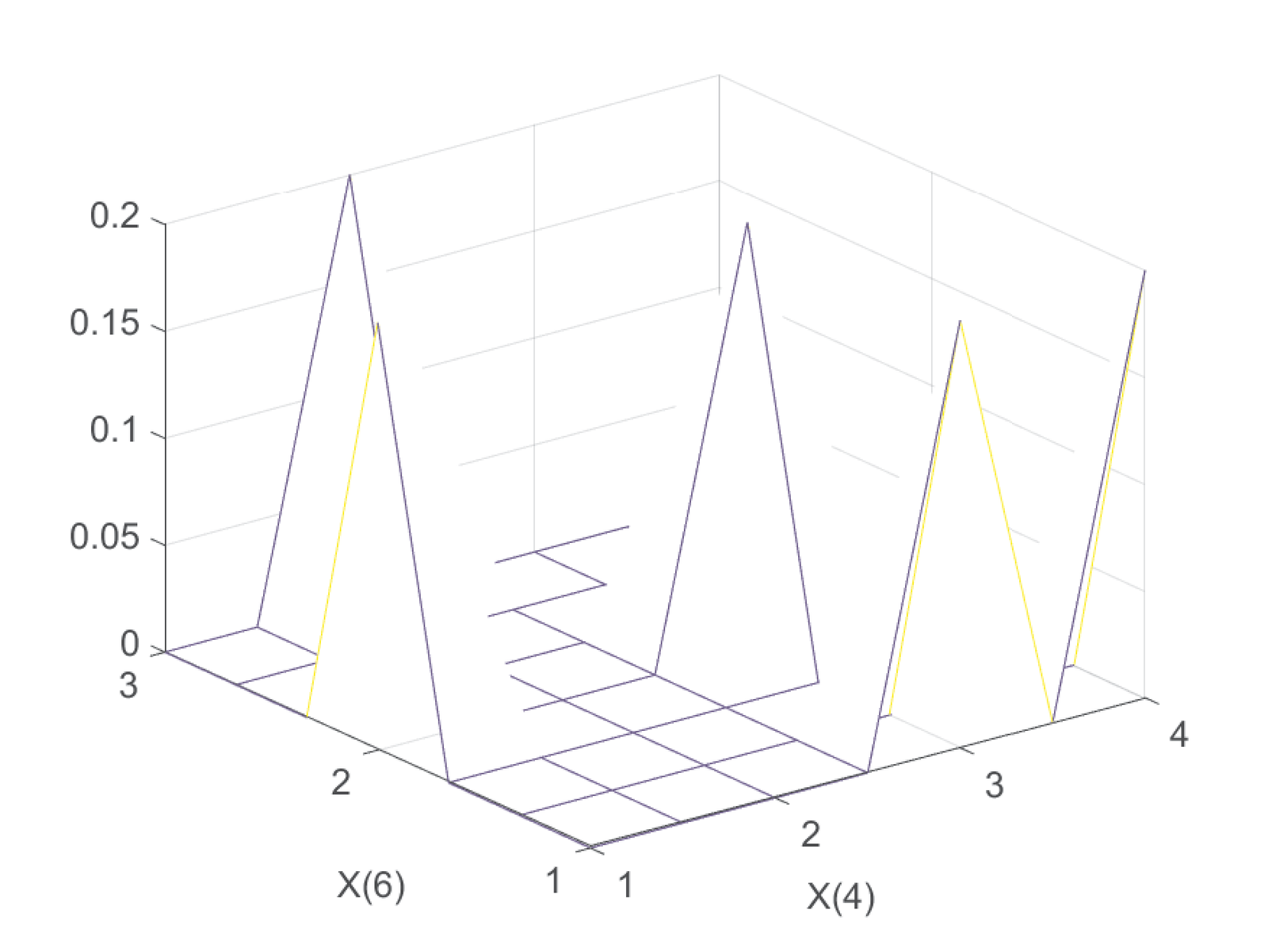
Figure A.11: Example of evaluating a random process at time instants $n = 4$ and $n = 6$ , which correspond to the values of two random variables $X [4]$ and $X [6]$ . There are only five pairs and each occurs once, hence a 0.2 estimated probability for all points.

The continuous-time random process $X (t)$ is similar to its discrete-time counterpart. Taking two different time values $t$ and $s$ leads to a pair of random variables, which can then be fully (statistically) characterized by a joint pdf function $f (X (t), X (s))$ . This can be extended to three or more time instants (random variables). Back to the discrete-time example, one can use a normalized two-dimensional histogram to estimate the joint PMF of $X [4]$ and $X [6]$ as illustrated in Figure A.12.

Figure A.12: Example of a joint pdf of the continuous random variables $X [4]$ and $X [6]$ .

This example aimed at distinguishing time and ensemble averages, which is fundamental to understand stochastic processes. $□$

Correlation Function and Matrix

Second-order moments of a random process involve statistics taken at two distinct time instants. Two of them are the correlation and covariance functions, which are very useful in practice.

As discussed in Section 1.10, the correlation function is an extension of the correlation concept to random signals generated by stochastic processes. The autocorrelation function (ACF)

R_{X} (s, t) = 𝔼 [X (s) X (t)]

(A.70)

is the correlation between random variables $X (s)$ and $X (t)$ at two different points $s$ and $t$ in time of the same random process. Its purpose is to determine the strength of relationship between the values of the signal occurring at two different time instants. For simplicity, it is called $R_{X} (s, t)$ instead of $R_{XX} (s, t)$ .

A discrete-time version of Eq. (A.70) is

R_{X} [n_{1}, n_{2}] = 𝔼 [X [n_{1}] X [n_{2}]],

(A.71)

where $n_{1}$ and $n_{2}$ are two “time” instants.

Specially for discrete-time processes, it is useful to organize autocorrelation values in the form of an autocorrelation matrix.

Example A.3. Calculating and visualizing the autocorrelation matrix (not assuming stationarity). Stationarity is a concept that will be discussed in the sequel (Appendix A.20.0.0). Calculating and visualizing autocorrelation is simpler when the process is stationary. But in this example, this property is not assumed and the autocorrelation is obtained for a general process.

Listing A.6 illustrates the estimation of $R_{X} [n_{1}, n_{2}]$ for a general discrete-time random process.⁵

Listing A.6: MatlabOctaveFunctions/ak_correlationEnsemble.m

1function [Rxx,n1,n2]=ak_correlationEnsemble(X, maxTime) 
2% function [Rxx,n1,n2]=ak_correlationEnsemble(X, maxTime) 
3%Estimate correlation for non-stationary random processes using 
4%ensemble averages (does not assume ergodicity). 
5%Inputs:  - X, matrix representing discrete-time process realizations 
6%           Each column is a realization of X. 
7%         - maxTime, maximum time instant starting from n=1, which 
8%           corresponds to first row X(1,:). Default: number of rows. 
9%Outputs: - Rxx is maxTime x maxtime and Rxx[n1,n2]=E[X[n1] X*[n2]] 
10%         - n1,n2, lags to properly plot the axes. The values of 
11%           n1,n2 are varied from 1 to maxTime. 
12[numSamples,numRealizations] = size(X); %get number of rows and col. 
13if nargin==1 
14    maxTime = numSamples; %assume maximum possible value 
15end 
16Rxx = zeros(maxTime,maxTime); %pre-allocate space 
17for n1=1:maxTime 
18    for n2=1:maxTime %calculate ensemble averages 
19        Rxx(n1,n2)=mean(X(n1,:).*conj(X(n2,:))); %ensemble statistics 
20        %that depends on numRealizations stored in X 
21    end 
22end

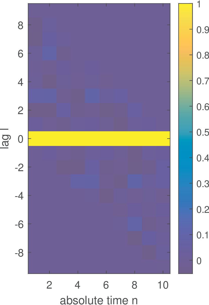
Figure A.13 was created with the command ak_correlationEnsemble(victories) and shows the estimated correlation for the data in Figure A.10 of Example A.2. The data cursor indicates that $R_{X} [1, 1] = 2.8$ because for $n = 1$ the random variables of the five realizations are $[2, 3, 0, 0, 1]$ . In this case, $R_{X} [1, 1] = 𝔼 [X {[1]}^{2}] \approx (4 + 9 + 1) ∕ 5 = 2.8$ . Similar calculation leads to $R_{X} [1, 7] = 𝔼 [X [1] X [7]] \approx 4.4$ because in this case the products victories(1,:).*victories(7,:) are [6, 12, 0, 0, 4], which have an average of 4.4.

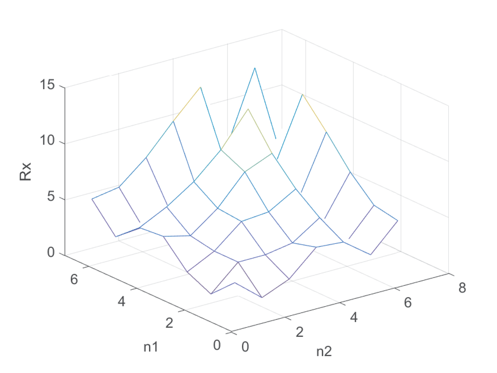
Figure A.13: Correlation for data in matrix victories.

Figure A.14 presents an alternative view of Figure A.13, where the values of the z-axis are indicated in color. The two datatips indicate that $R_{x} [1, 2] = 0.8$ and $R_{x} [3, 5] = 6.6$ (these are the values identified by Index for the adopted colormap, and the associated color is also shown via its RGB triple).

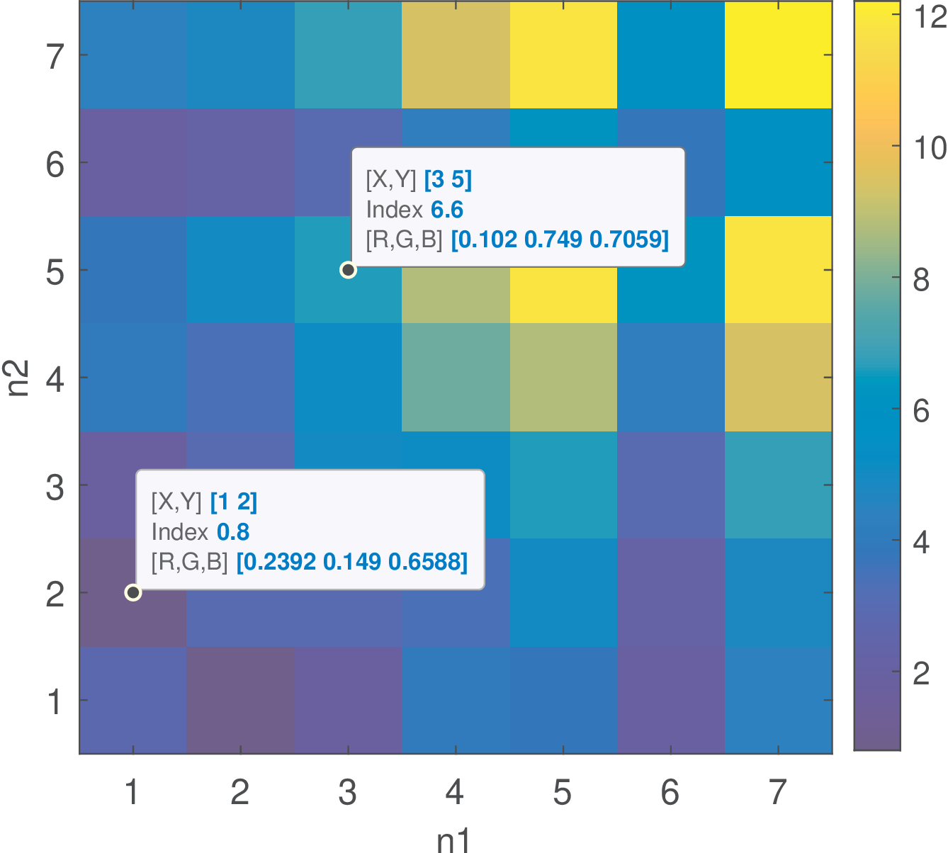
Figure A.14: Version of Figure A.13 using an image.

For real-valued processes, the autocorrelation is symmetric, as indicated in Figure A.13 and Figure A.14, while it would be Hermitian for complex-valued processes. $□$

Two time instants: both absolute or one absolute and a relative (lag)

When characterizing second-order moments of a random process, instead of using two absolute time instants, it is sometimes useful to make one instant as a relative “lag” with respect to the other. For example, take two absolute instants $t = 4$ and $s = 7$ in Eq. (A.70). Alternatively, the same pair of instants can be denoted by considering $t = 4$ as the absolute time that provides the reference instant and a lag $τ = s - t = 3$ indicating that the second instant is separated by 3 from the reference.

Using this scheme, Eq. (A.70) can be written as

R_{X} (t, τ) = 𝔼 [X (t + τ) X (t)] .

(A.72)

Similarly, Eq. (A.71) can be denoted as

R_{X} [n, l] = 𝔼 [X [n] X [n + l]],

(A.73)

with $n_{1} = n$ and $n_{2} = n + l$ , where $l$ is the lag in discrete-time.

Example A.4. Contrasting two different representations of autocorrelations. Figure A.13 is a graph that corresponds to Eq. (A.71), with two absolute time instants. When using the alternative representation of Eq. (A.73), with a lag, the resulting matrix is obtained by rearranging the elements of the autocorrelation matrix. Figure A.15 compares the two cases. Note that the name autocorrelation matrix is reserved for the one derived from Eq. (A.71) (and Eq. (A.70)) that is, for example, symmetric.

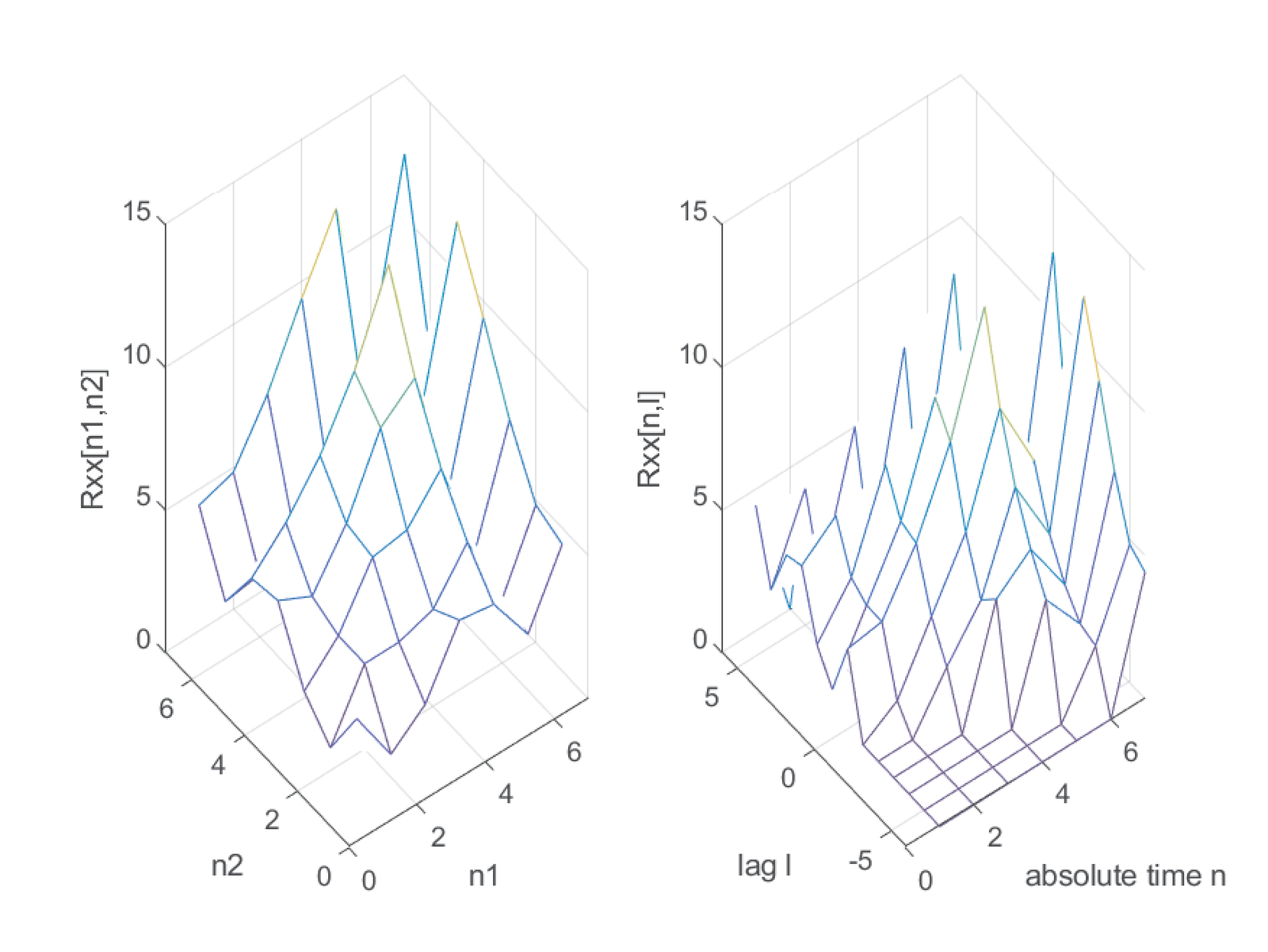
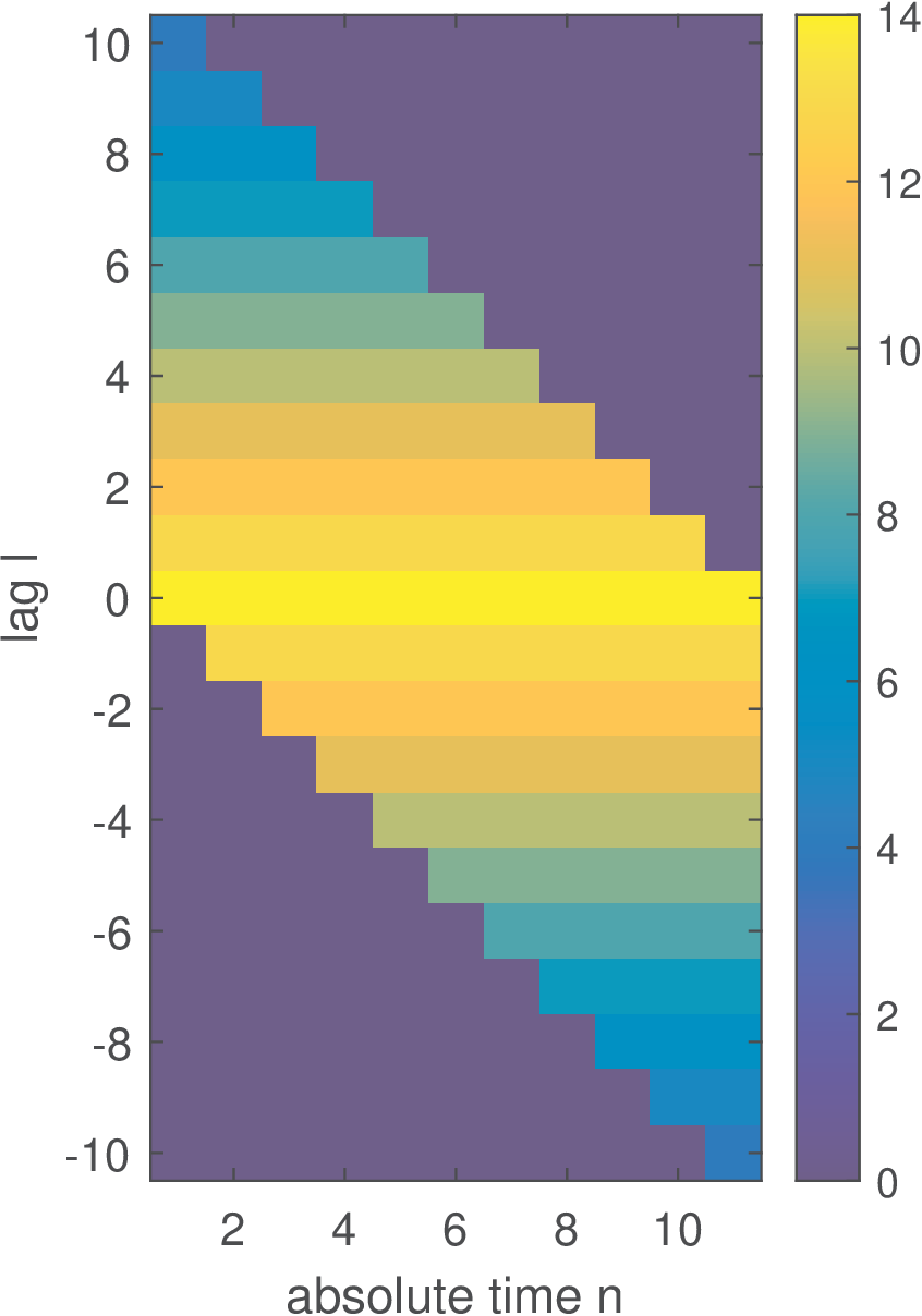
Figure A.15: Comparison between the 3-d representation of the autocorrelation matrix in Figure A.13 and the one using lags as in Eq. (A.73).

Figure A.16 is an alternative view of Figure A.15, which makes visualization easier. It better shows that Eq. (A.73) leads to shifting the column of the autocorrelation matrix (Figure A.13) corresponding to each value $n = n_{1}$ of interest.

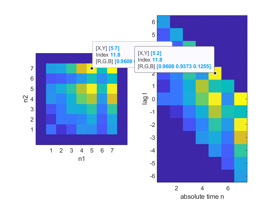
Figure A.16: Comparison between autocorrelation representations using images instead of 3-d graphs as in Figure A.15.

Properties such as the symmetry of the autocorrelation matrix may not be so evident from the right-side representation of Figure A.16 as in the left-side representation, but both are useful in distinct situations. $□$

Covariance matrix

Similar to autocorrelation functions, it is possible to define covariance functions that expand the definition for random variables such as Eq. (1.47) and take as arguments two time instants of a random process. For example, for a complex-valued discrete-time process the covariance is

c_{X} [n, l] = 𝔼 [(X [n] - μ [n]) {(X [n + l] - μ [n + l])}^{*}] .

(A.74)

Stationarity, cyclostationarity and ergodicity

A random process is a powerful model. Hence, an important question is what information is necessary to fully characterize it. Take the $7 \times 5$ matrix in Example A.2: this data does not fully characterize the random process because it consists of only five realizations (tossing a coin five times does not allow to estimate its probability of heads robustly). We would need an infinite number of realizations if we insist in characterizing it in a tabular form. The most convenient alternative is to describe it through pdfs. We should be able to indicate, for all time $t$ , the pdf of $X (t)$ . Besides, for each time pair $(t, s)$ , the joint pdf $f (X (t), X (s))$ should be known. The same for the pdf $f (X (t), X (s), X (r))$ of each triple $(t, s, r)$ and so on. It can be noted that a general random process requires a considerable amount of statistics to be fully described. So, it is natural to define particular and simpler cases of random processes as discussed in the sequel.

An important property of a random process is the stationarity of a statistics, which means this statistics is time-invariant even though the process is random. More specifically, a process is called $n$ -th order stationary if the joint distribution of any set of $n$ of its random variables is independent of absolute time values, depending only on relative time.

A first-order stationary process has the same pdf $f (X (t)), \forall t$ (similar is valid for discrete-time). Consequently, it has a constant mean

𝔼 [X (t)] = μ, \forall t,

(A.75)

constant variance and other moments such as $𝔼 [X^{4} (t)]$ .

A second-order stationary process has the same joint pdf $f (X (t), X (s)) = f (X (t + τ), X (s + τ)), \forall t, s$ . Consequently, its autocorrelation is

R_{X} (τ) = 𝔼 [X (t + τ) X (t)],

(A.76)

where the time difference $τ = s - t$ is called the lag and has the same unit as $t$ in $X (t)$ . Note that, in general, $R_{X} (t, τ)$ of Eq. (A.72) depends on two parameters: $t$ and $τ$ . However, for a stationary process, Eq. (A.76) depends only on the lag $τ$ because, given $τ$ , $R_{X} (t, τ) = R_{X} (τ)$ is the same for all values of $t$ .

Similarly, if a discrete-time process is second-order stationary, $R_{X} [n, l]$ Eq. (A.73) can be simplified to

R_{X} [l] = 𝔼 [X [n] X [n + l]],

(A.77)

where $l = n_{2} - n_{1}$ is the lag.

A third-order stationary process has joint pdfs $f (X (t_{1}), X (t_{2}), X (t_{3}))$ that do not depend on absolute time values $(t_{1}, t_{2}, t_{3})$ and so on. A random process $X (t)$ is said to be strict-sense stationary (SSS) or simply stationary if any joint pdf $f (X (t_{1}), \dots, X (t_{n}))$ is invariant to a translation by a delay $τ$ . A random process with realizations that consist of i. i. d. random variables (called an i. i. d. process) is SSS. A random process that is not SSS is referred to as a non-stationary process even if some of its statistics have the stationarity property.

The SSS process has very stringent requirements, which are hard to verify. Hence, many real-world signals are modeled as having a weaker form of stationarity called wide-sense stationarity.

Basically, a wide-sense stationary (WSS) process has a mean that does not vary over time and an autocorrelation that does not depend on absolute time, as indicated in Eq. (A.75) and Eq. (A.76), respectively. Broadly speaking, wide-sense theory deals with moments (mean, variance, etc.) while strict-sense deals with probability distributions. Note that SSS implies WSS but the converse is not true in general, with Gaussian processes being a famous exception.

For example, the process corresponding to Figure A.13 is not WSS: its autocorrelation does not depend only on the time difference $τ$ .

Example A.5. The autocorrelation matrix of a WSS process is Toeplitz. For a WSS process, elements $R_{X} (i, j)$ of its autocorrelation matrix depend only on the absolute difference $| i - j |$ and, therefore, the matrix is Toeplitz. In this example, the function toeplitz.m is used to visualize the corresponding autocorrelation matrix as an image. For example, the command Rx=toeplitz(1:4) generates the following real-valued matrix:

 Rx=[1     2     3     4
     2     1     2     3
     3     2     1     2
     4     3     2     1].

Usually, the elements of the main diagonal correspond to $R_{X} (0) = 𝔼 [X^{2} [n]]$ .

To visualize a larger matrix, Figure A.17 was generated with Rxx=toeplitz(14:-1:4).

Figure A.17: Representation of a WSS autocorrelation matrix that depends only on the lag $l$ .

Given the redundancy in Figure A.17, one can observe that for a WSS, it suffices to describe $R_{X} (l)$ for each value of the lag $l$ . $□$

A cyclostationary process is a non-stationary process having statistical properties that vary periodically (cyclically) with time. In some sense it is a weaker manifestation of a stationarity property. Cyclostationary processes are further discussed in Appendix A.20.1.

A given statistics (variance, autocorrelation, etc.) of a random process is ergodic if its time average is equal to the ensemble average. For example, an i. i. d. random process is ergodic in the mean.⁶ And, loosely speaking, a WSS is ergodic in both mean and autocorrelation if its autocovariance decays to zero.⁷

A process could be called “ergodic” if all ensemble and time averages are interchangeable. However, it is more pedagogical to consider ergodicity as a property of specific statistics, and always inform them.⁸ Even non-stationary or cyclostationary processes can be ergodic in specific statistics such as the mean. Figure A.18 depicts the suggested taxonomy of random processes using a Venn diagram.

Figure A.18: Suggested taxonomy of random processes. SSS are sometimes called stationary and all processes that are not SSS are called non-stationary.

Example A.6. Polar and unipolar bitstreams modeled as WSS processes. This example is based on processes used in digital communications to represent sequences of bits. Note that, after these bit streams are upsampled in order to create line codes, they become cyclostationary processes. This issue is discussed in Appendix A.20.1, while here the sequences are not upsampled.

Figure A.19 illustrates two processes for which the main diagonal $R_{X} [1, 1] = R_{X} [2, 2] = R_{X} [3, 3] \dots$ has the same values. The process (a) (left-most) is called a unipolar line code and consists of sequences with equiprobable values 0 and 1, while for the second process (called polar) the values are $- 1$ and 1.

For the unipolar and polar cases, the theoretical correlations $R_{X} [n_{1}, n_{2}]$ for $n_{1} = n_{2}$ are 0.5 and 1, respectively. The result is obtained by observing that $R_{X} [n_{1}, n_{2}] = R_{X} [n_{1}, n_{1}] = 𝔼 [X {[n_{1}]}^{2}]$ and for the unipolar case, $X {[n_{1}]}^{2}$ is 0 or 1. Because the two values are equiprobable, $𝔼 [X {[n_{1}]}^{2}] = 0.5$ . For the polar case, $X {[n_{1}]}^{2} = 1$ always and $𝔼 [X {[n_{1}]}^{2}] = 1$ . The values of $R_{X} [n_{1}, n_{2}]$ for $n_{1} \neq n_{2}$ are obtained by observing the values of all possible products $X [n_{1}] X [n_{2}]$ . For the unipolar case, the possibilities are $0 \times 0 = 0$ , $0 \times 1 = 0$ , $1 \times 0 = 0$ and $1 \times 1 = 1$ , all with probability 1/4 each. Hence, for this unipolar example, $𝔼 [X [n_{1}] X [n_{2}]] = (3 \times 0 + 1 \times 1) ∕ 4 = 0.25, n 1 \neq n 2$ . For the polar case, the possibilities are $- 1 \times - 1 = 1$ , $- 1 \times 1 = 1$ , $1 \times - 1 = - 1$ and $1 \times 1 = 1$ , all with probability 1/4 each. Hence, for this polar example, $𝔼 [X [n_{1}] X [n_{2}]] = (2 \times - 1 + 2 \times 1) ∕ 4 = 0, n 1 \neq n 2$ .

In summary, for the polar code $R_{X} [n_{1}, n_{2}] = 1$ for $n_{1} = n_{2}$ and 0 otherwise. For the unipolar code, $R_{X} [n_{1}, n_{2}] = 0.5$ for $n_{1} = n_{2}$ and 0.25 otherwise.

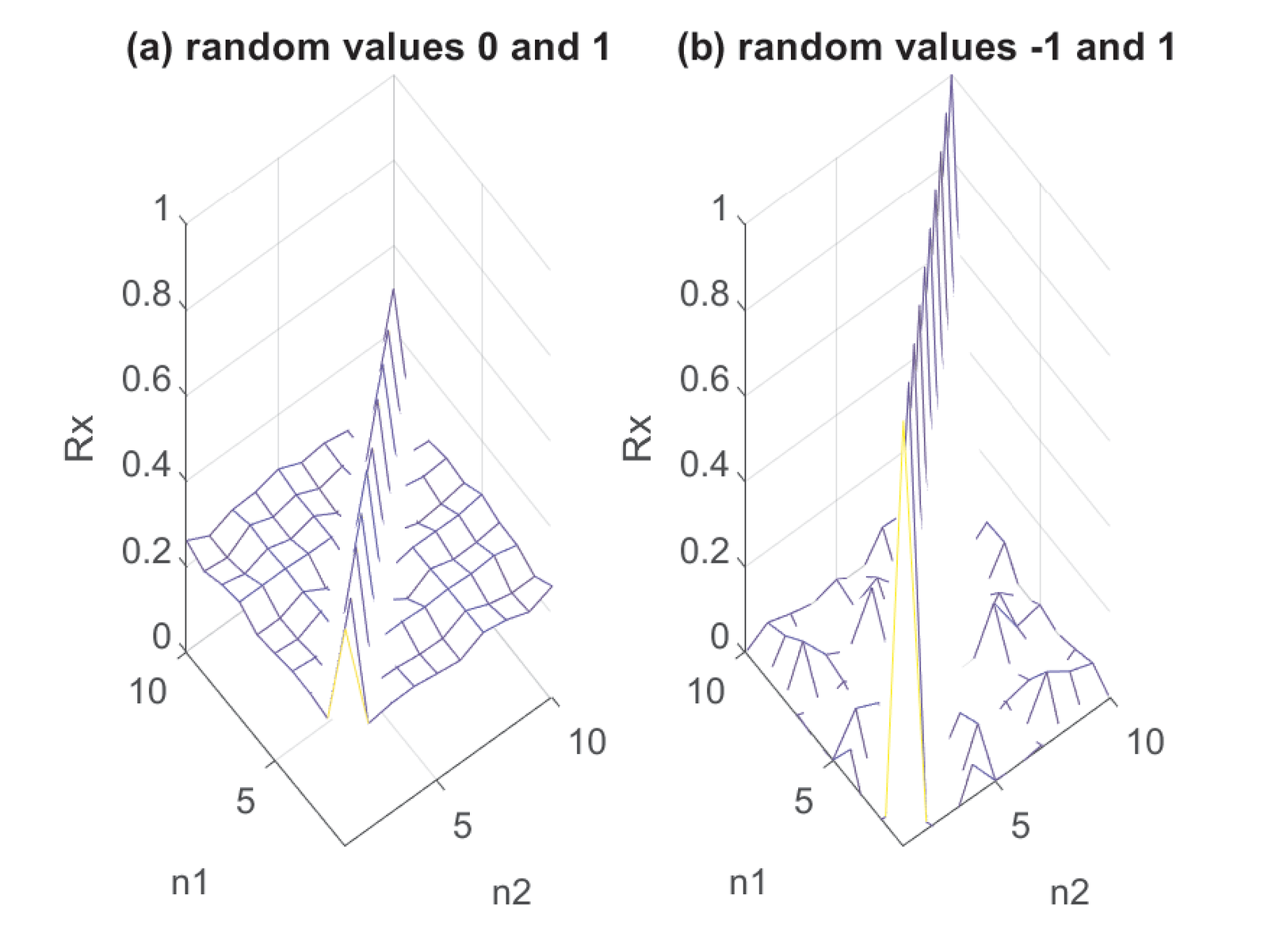
Figure A.19: Correlation for random sequences with two equiprobable values: a) values are 0 and 1 (unipolar), b) values are $- 1$ and 1 (polar).

A careful observation of Figure A.19 indicates that two dimensions are not necessary and it suffices to describe $R_{X} [l]$ as in Eq. (A.73). As discussed previously, in the case of WSS processes, the correlation depends only on the difference between the “time” instants $n_{1}$ and $n_{2}$ . Figure A.20 emphasizes this aspect using another representation for the polar case in Figure A.19.

Figure A.20: Alternative representation of the correlation values for the polar case of Figure A.19.

Because the polar and unipolar processes that were used to derive Figure A.19 are WSS, Listing A.7 can be used to take advantage of having $R_{X} [n_{1}, n_{2}]$ depending only on the lag and convert this matrix to an array $R_{X} [l]$ .

Listing A.7: MatlabOctaveFunctions/ak_convertToWSSCorrelation.m

1function [Rxx_tau, lags] = ak_convertToWSSCorrelation(Rxx) 
2% function [Rxx_tau,lags]=ak_convertToWSSCorrelation(Rxx) 
3%Convert Rxx[n1,n2] into Rxx[k], assuming process is 
4%wide-sense stationary (WSS). 
5%Input: Rxx -> matrix with Rxx[n1,n2] 
6%Outputs: Rxx_tau[lag] and lag=n2-n1. 
7[M,N]=size(Rxx); %M is assumed to be equal to N 
8lags=-N:N; %lags 
9numLags = length(lags); %number of lags 
10Rxx_tau = zeros(1,numLags); %pre-allocate space 
11for k=1:numLags; 
12    lag = lags(k); counter = 0; %initialize 
13    for n1=1:N 
14        n2=n1+lag; %from: lag = n2 - n1 
15        if n2<1 || n2>N %check 
16            continue; %skip if out of range 
17        end 
18        Rxx_tau(k) = Rxx_tau(k) + Rxx(n1,n2); %update 
19        counter = counter + 1; %update 
20    end 
21    if counter ~= 0 
22        Rxx_tau(k) = Rxx_tau(k)/counter; %normalize 
23    end 
24end

Figure A.21 was generated using Listing A.7 for the data in Figure A.19.

Figure A.21: One-dimensional ACF $R_{X} [l]$ for the data corresponding to Figure A.19 (unipolar and polar codes).

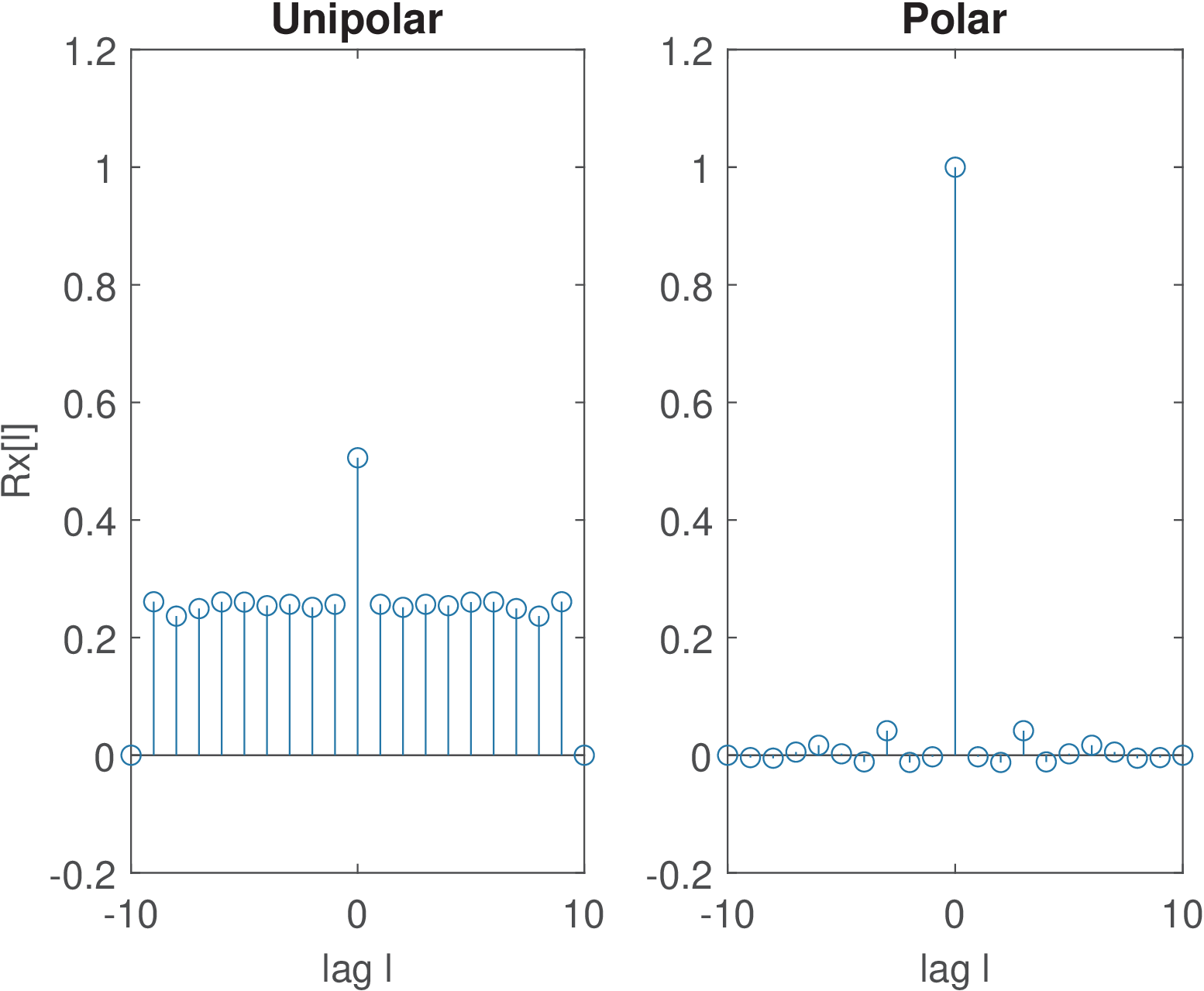
If ergodicity can be assumed, a single realization of the process can be used to estimate the ACF. Figure A.22 was generated using the code below, which generates a single realization of each process:

1numSamples=1000; 
2Xunipolar=floor(2*rand(1,numSamples)); %r.v. 0 or 1 
3[Rxx,lags]=xcorr(Xunipolar,9,'unbiased');%Rxx for unipolar 
4subplot(121); stem(lags,Rxx) title('Unipolar'); 
5Xpolar=2*[floor(2*rand(1,numSamples))-0.5]; %r.v. -1 or 1 
6[Rxx,lags]=xcorr(Xpolar,9,'unbiased'); %Rxx for polar code 
7subplot(122); stem(lags,Rxx) title('Polar');

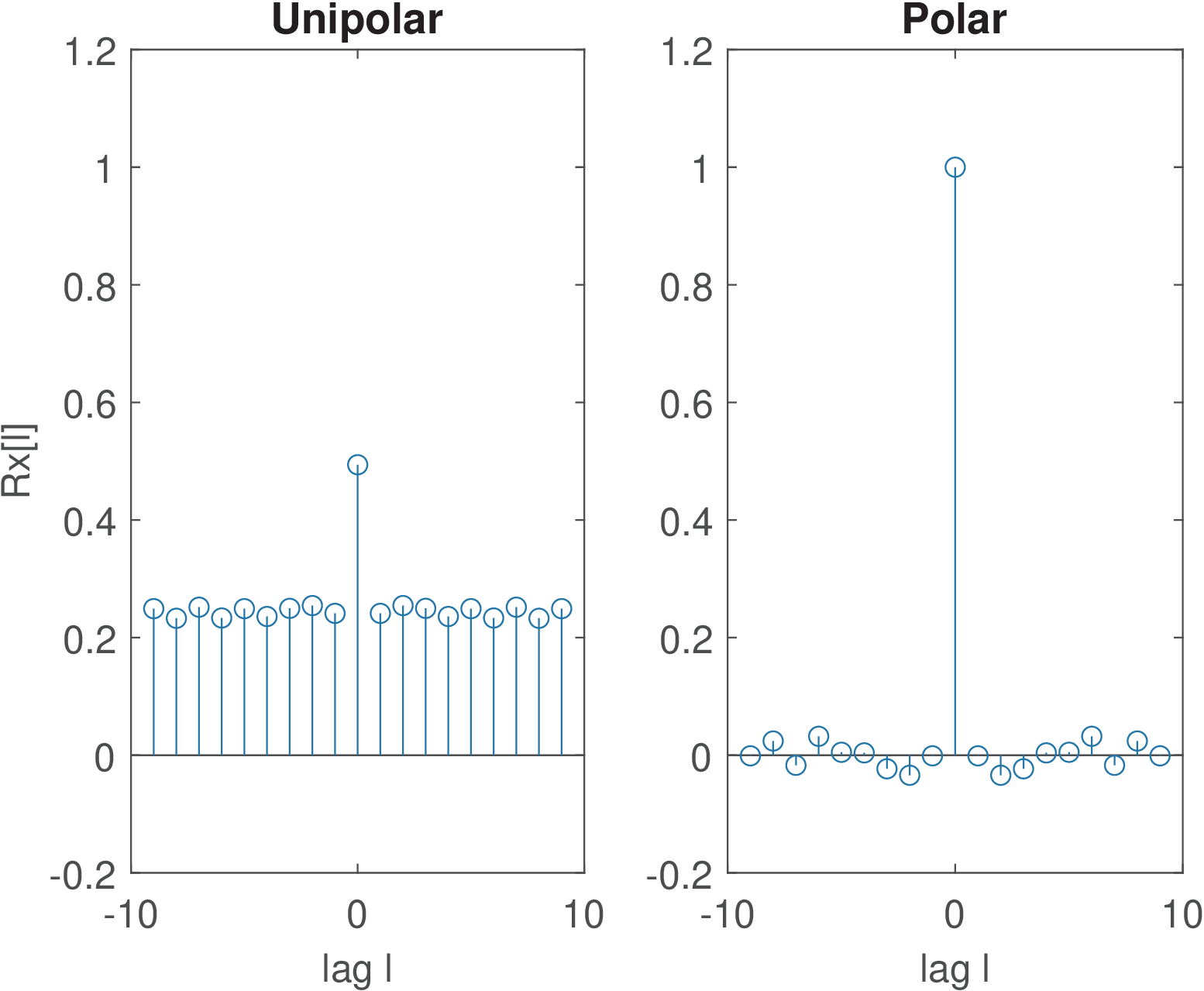
Increasing the number of samples to numSamples=1e6 achieves estimation errors smaller than in Figure A.22.

Figure A.22: ACF estimated using ergodicity and waveforms with 1,000 samples for each process. The theoretical values are 0.25 and 0.5 (at $l = 0$ ) for unipolar, while for polar these values are 0 and 1.

□

A.20.1 Cyclostationary random processes

This section aims at providing some intuition about cyclostationarity. More information can be found e. g. in [Gia99, Ant07, Gar91].

A discrete-time process $X [n]$ is wide-sense cyclostationary (WSC) if, and only if, exists an integer period $P > 0$ such that the mean and correlation are periodic (consequently, the covariance is periodic too), as summarized by:

\begin{align} μ_{X} [n] & = μ_{X} [n + P] and \\ R_{X} [n, l] & = R_{X} [n + P, l] . & (A.78) \end{align}

Note that the correlation is periodic but a cyclostationary process generates realizations that are random and not periodic. To avoid confusion, the period $P$ in Eq. (A.78) of a WSC process is referred to as its cycle.

Because WSC are more common than strict-sense cyclostationary processes, the term cyclostationary is assumed here to correspond to a WSC (wide, not strict sense), as adopted in [Gia99], which is the main reference for the discussion presented in the sequel. In order to better understand WSC processes, it is useful to review the concepts of non-stationary processes in Appendix A.20 and get familiar with representations such as the ones in Figure A.15 and Figure A.16. While WSS processes have autocorrelations depending only on one parameter, the lag $l$ , WSC correlations depend on two parameters ( $R_{X} [n, l]$ ) and this is a key factor for the following discussion.

Note that Eq. (A.78) implies the correlation $R_{X} [n, l]$ in Eq. (A.73) is periodic in $n$ for each “lag” $l$ . In other words, given a lag value $l_{0}$ , the time-series $R_{X} [n, l_{0}]$ over the “absolute time instant” $n$ is periodic. Hence, it can be represented using a DTFS in which the Fourier coefficients $C_{X} [k, l]$ are called cyclic correlations. Therefore, when $R_{X} [n, l]$ has a period of $P$ samples over $n$ , the following Fourier pair can be used:

R_{X} [n, l] = \sum_{k = 0}^{P - 1} C_{X} [k, l] e^{j \frac{2 π}{P} nk} \Leftrightarrow C_{X} [k, l] = \frac{1}{P} \sum_{n = 0}^{P - 1} R_{X} [k, l] e^{- j \frac{2 π}{P} nk} .

(A.79)

$R_{X} [n, l]$ is also called time-varying correlation and instantaneous correlation.

As explained in [Gia99], sampling a continuous-time periodic signal may lead to an almost periodic signal for which Eq. (1.21) does not hold. This occurs in the so-called wide-sense almost cyclostationary processes, in which $R_{X} [n, l]$ has the following generalized Fourier series:

R_{X} [n, l] = \sum_{α_{k} \in C} C_{X} [α_{k}, l] e^{j α_{k} n} \Leftrightarrow C_{X} [α_{k}, l] = lim_{N \to \infty} \frac{1}{N} \sum_{n = 0}^{P - 1} R_{X} (k, l) e^{- j α_{k} n},

(A.80)

where $C$ is the set $C = {α_{k} : C_{X} [α_{k}, l] \neq 0, - π \leq α_{k} < π}$ of cycles.

The estimation of both $C_{X} [k, l]$ and $C_{X} [α_{k}, l]$ is often done with FFTs and, consequently, both periodic and almost periodic realizations are treated similarly. Hereafter, the notation $C_{X} [α_{k}, l]$ is also adopted for $C_{X} [k, l]$ .

For a given cycle $α_{k}$ , the evolution of $C_{X} [α_{k}, l]$ over the lags $l$ can be interpreted over frequency using its DTFT to define the cyclic spectrum:

S_{X} (α_{k}, Ω) = \sum_{l = - \infty}^{\infty} C_{X} [α_{k}, l] e^{- j Ω l} .

(A.81)

In summary, while stationary discrete-time signals are analyzed using PSDs in frequency-domain ( $Ω$ ) and time-invariant correlations in lag-domain ( $l$ ), non-stationary signals include also the time ( $n$ ) and cycle ( $α$ ) domains. Figure A.23 illustrates the relations.

Figure A.23: Functions used to characterize cyclostationary processes. FS stands for “generalized Fourier series”, useful for representing “almost periodic” discrete-time signals (Adapted from Fig. 17.1 of [Gia99] to include the notation adopted in this text and the one widely used by [Gar91]).

As further discussed in Section A.20.3, a cyclostationary process can be converted into a WSS through the “uniform shift” or “uniformly randomizing the phase” [Gia99].

The following example aims at making these concepts more concrete.

Example A.7. Example: WGN modulated by sinusoid. Assume $ν [n]$ represents a realization of an i. i. d. white Gaussian noise process with variance $σ^{2}$ . Each realization is modulated by a carrier of frequency $Ω_{c}$ and phase $ϕ$ (both in radians) leading to⁹

x [n] = ν [n] cos (Ω_{c} n + ϕ) .

(A.82)

The top plot in Figure A.24 illustrates a single realization of $x [n]$ , as generated by Listing A.8. It can be seen that the sinusoid is “buried” in noise. All M=5000 realizations are stored in matrix X. The ensemble variance for each “time” instant $n$ is shown in the bottom plot of Figure A.24, indicating that the variance has a period $P ∕ 2$ (in this case, 15 samples, given that P=30) because it depends on the absolute value of the sinusoid amplitude at instant $n$ . This can be also seen from the correlation of $x [n]$ over time, as discussed in the sequel.

Listing A.8: MatlabOctaveCodeSnippets/snip_appprobability_modulatednoise.m

1M=5000; %number of realizations for ensemble statistics 
2N=1000; %number of samples of each realization 
3P=30; %sinusoid period (in samples) 
4X=zeros(N,M); %pre-allocate space 
5Wc=2*pi/P; Phc=pi/5; %carrier frequency and phase, both in radians 
6n=0:N-1; carrier=transpose(cos(Wc*n+Phc)); %same for all realizations 
7%carrier(carrier>0)=1; carrier(carrier<0)=-1; %if wants square wave 
8for m=1:M %for each realization 
9    X(:,m)=randn(N,1).*carrier; %WGN modulated by sinusoidal carrier 
10end

Figure A.24: Single realization $x [n]$ of Eq. (A.82) (top) and the ensemble variance over time (bottom plot), which has a period of $P ∕ 2 = 15$ samples.

From Eq. (A.73), the correlation of $x [n]$ is

\begin{align} R_{X} [n, l] & = 𝔼 [ν [n] cos (Ω_{c} n + ϕ) ν [n + l] cos (Ω_{c} (n + l) + ϕ)] \\ = cos (Ω_{c} n + ϕ) cos (Ω_{c} (n + l) + ϕ) 𝔼 [ν [n] ν [n + l]] = {cos}^{2} (Ω_{c} n + ϕ) σ^{2} δ [l] \\ = \frac{σ^{2}}{2} (1 + cos (2 Ω_{c} n + 2 ϕ)) δ [l], & (A.83) \end{align}

which is depicted in Figure A.25(b). The value of $δ [l]$ is 1 for all $n$ when $l = 0$ and zero otherwise. Note that Figure A.25(a) is the alternative representation with a pair of absolute time instants $[n_{1}, n_{2}]$ .

Figure A.25: Cyclostationary analysis of the modulated white Gaussian noise.

Eq. (A.83) is non-zero only at $l = 0$ , where it is a squared cosine ${cos}^{2} (Ω_{c} n) σ^{2}$ . Hence, from Eq. (A.8), its cyclic correlation is $C_{X} [α_{k}, l] = \frac{σ^{2}}{2} δ [α] + \frac{σ^{2}}{4} (δ [α + 2 Ω_{c}] + δ [α - 2 Ω_{c}])$ . And the cyclic spectrum is obtained by a DTFT for each cycle, which leads to the DC levels in Figure A.25(d).

Eq. (A.82) can be modified to $x [n] = ν [n] p [n]$ , where $p [n]$ is a generic periodic signal. In this case, $C_{X} [α_{k}, l] = c_{k} σ^{2} δ [l]$ , where $c_{k}$ is the Fourier coefficient of $| p [n] |^{2}$ , as discussed in [Ant07].

Listing A.9 indicates how the sinusoid frequency and phase can be obtained using the realizations in matrix X created by Listing A.8.

Listing A.9: MatlabOctaveCodeSnippets/snip_appprobability_cyclo_analysis_ensemble.m

1snip_appprobability_modulatednoise %generate modulated WGN 
2alphaFFTLength=3*P; %P is the period, a multiple of P avoids leakage 
3[Cxx,alphas,lags] = ak_cyclicCorrelationEnsemble(X, alphaFFTLength); 
4onlyPositiveCycles=1; exclude0Alpha=1; %take only alpha>0 in account 
5[peakValue,peakAlpha,peakLag] = ak_peakOfCyclicCorrelation(Cxx, ... 
6    alphas,lags,exclude0Alpha,onlyPositiveCycles); %get the peak 
7WEstimated=peakAlpha/2; %estimated frequency in rad 
8phaseEstimated = angle(peakValue)/2; %phase in rad 
9phaseOffset=wrapToPi(Phc) - wrapToPi(phaseEstimated); %force [-pi,pi] 
10periodEstimated=round(2*pi/WEstimated); %estimate period (samples)

It should be noted that the phase estimation is highly sensitive to the value of alphaFFTLength (relatively, the frequency estimation is more robust). The reader is invited to modify this value and observe the estimation errors. As an example, the following output was obtained with Listing A.9:

Peak value=0.25187*exp(1.2545j)
Period:  Correct=30, Estimated=30 (samples)
Cycle:  Correct=0.20944, Estimated=0.20944(rad). Error=2.7756e-17
Phase:  Correct=0.62832, Estimated=0.62724(rad). Error=0.0010821

In this example the cyclic correlation was obtained with ensemble statistics. The following discussion concerns estimation using a single realization. $□$

When it is feasible to assume ergodicity in the autocorrelation of a WSC, the estimation can be done with a single realization of $N$ samples. In this case and assuming a complex-valued $x [n]$ signal, an estimator for the cyclic correlation is:¹⁰

Ĉ_{X} [α_{k}, l] = \frac{1}{N} \sum_{n = 0}^{N - l - 1} x [n] x^{*} [n + l] e^{- j α_{k} n}, l \geq 0 .

(A.84)

For negative $l$ , one can use $Ĉ_{X} [α_{k}, - l] = Ĉ_{X}^{*} [α_{k}, l] e^{j α_{k} l}$ .

Example A.8. Example: WGN modulated by sinusoid using a single realization. Listing A.10 estimates the cyclic spectrum using a single realization of Example A.7.

Listing A.10: MatlabOctaveCodeSnippets/snip_appprobability_cyclo_analysis.m

1snip_appprobability_modulatednoise %generate modulated WGN 
2x=X(:,1); %take one realization 
3maxTau=3*P; %maximum lag value (P is the sinusoid period) 
4numCycles=4*P; %the cycle resolution is then 2*pi/numCycles 
5[Cxx,alphas,lags]=ak_cyclicCorrelation(x,maxTau,numCycles);

The output of Listing A.10 in this case is

Peak value=0.24393*exp(1.3427j)
Period:  Correct=30, Estimated=30 (samples)
Cycle:  Correct=0.20944, Estimated=0.20944(rad). Error=0
Phase:  Correct=0.62832, Estimated=0.67133(rad). Error=-0.043013

Listing A.10 is similar to Listing A.9, but estimates the cyclic correlation $C_{X} [α_{k}, l]$ from a single realization instead of ensemble statistics. The main functions for these codes are ak_cyclicCorrelation.m and ak_cyclicCorrelationEnsemble.m, respectively. $□$

In both Listing A.10 and Listing A.9, the duration of the signals was carefully controlled to improve accuracy. More sophisticated algorithms use windowing or estimate the cyclic spectrum directly, via periodograms.

Example A.9. Example: Cyclic spectrum via periodograms. The cyclic spectrum $S_{X} (α_{k}, Ω)$ of Eq. (A.81) can be obtained by first estimating the cyclic correlation $C_{X} [α_{k}, l]$ as in ak_cyclicSpectrum.m, which was used to obtain Figure A.25(d). Alternatively, $S_{X} (α_{k}, Ω)$ can be directly estimated via periodograms [Ant07, GG98].

Listing A.11 estimates the cyclic spectrum using a single realization of the modulated WGN in Example A.7.

Listing A.11: MatlabOctaveCodeSnippets/snip_appprobability_cyclo_spectrum_periodograms

1P=30; %sinusoid period (in samples) 
2N=1e3*P; %number of samples of this realization (force multiple of P) 
3Wc=2*pi/P; Phc=pi/5; %carrier frequency and phase, both in radians 
4n=0:N-1; carrier=transpose(cos(Wc*n+Phc)); %same for all realizations 
5x=randn(N,1).*carrier; %WGN modulated by sinusoidal carrier 
6L = length(x);      % signal length 
7Nw = 128;           % window length 
8Nv = fix(2/3*Nw);   % block overlap 
9nfft = 2*Nw;        % FFT length 
10da = 1/L;           % cyclic frequency resolution (normalized freq) 
11cycleIndex = round(2*Wc/(2*pi*da)); %find the correct cycle 
12a1 = cycleIndex-20; % first cyclic freq. bin to scan (cycle a1*da) 
13a2 = cycleIndex+20; % last cyclic freq. bin to scan (cycle a2*da) 
14S = zeros(nfft,a2-a1+1); %pre-allocate space 
15for k = a1:a2; % Loop over all chose cyclic frequencies 
16    spectralObject = cps_w(x,x,k/L,nfft,Nv,Nw,'sym'); %cycle k/L 
17    S(:,k-a1+1) = spectralObject.S; %extract S(alpha,f) from object 
18end 
19alphas = 2*pi*da*(a1:a2); %get all cycles in rad 
20sumMagOverFreq=sum(abs(S)); %for each cycle, sum all magnitudes 
21indMax=find(sumMagOverFreq == max(sumMagOverFreq),1); 
22WEstimated=alphas(indMax)/2; %estimated frequency from cycle of peak 
23periodEstimated=round(2*pi/WEstimated); %period in samples 
24phaseEstimated=mean(angle(S(:,indMax)))/2;%half averaged peak's phase

Listing A.11 is based on the third-party function cps_w.m,¹¹ which allows calculating $S_{X} (α_{k}, Ω)$ for specific values of $α_{k}$ . This is handy when there is previous knowledge about the cycles of interest.

The output of Listing A.11 is:

Period:  Correct=30, Estimated=30 (samples)
Cycle:  Correct=0.20944, Estimated=0.20944(rad). Error=-2.7756e-17
Phase:  Correct=0.62832, Estimated=0.64059(rad). Error=-0.012276

Note that this relatively good result was obtained with N chosen as a multiple of P and, consequently, the sinusoid frequency Wc is a multiple of the cycle resolution da. Changing N from $30$ to $40$ thousand samples led to:

Period:  Correct=30, Estimated=30 (samples)
Cycle:  Correct=0.20944, Estimated=0.20947(rad). Error=-2.618e-05
Phase:  Correct=0.62832, Estimated=0.10469(rad). Error=0.52363

which has an significantly increased phase estimation error. Practical issues when estimating cyclostationary statistics are discussed, for example, in [Ant07]. $□$

A.20.2 Two cyclostationary signals: sampled and discrete-time upsampled

Cyclostationarity is discussed here in the context of digital communications. More specifically, two signals of interest with periodic statistics are:

m_{u} [n] and x_{s} (t),

(A.85)

which are generated, respectively, by the following processes:

the output $m_{u} [n]$ of an upsampler when its input $m [n']$ is a discrete-time WSS process;
the sampled signal $x_{s} (t)$ obtained by periodic sampling of a continuous-time WSS process.

The upsampler of the former case is discussed in Section 3.17, and its block diagram is repeated here for convenience:

m [n'] \to ↑ L \to m_{u} [n] .

The first goal of this discussion is to indicate that $m_{u} [n]$ is WSC (wide-sense cyclostationary) while $m [n']$ is WSS.

Example A.6 discusses that the input $m [n']$ is WSS and presents the corresponding autocorrelations $R_{m} [l]$ for a polar and unipolar binary signal. But, as informed in Section 3.17, the upsampling by $L$ is not a time-invariant operation and the output process cannot be assumed WSS in spite of the input being WSS. This fact can be confirmed by observing Figure A.26 and Figure A.27. Figure A.26 shows that the amplitudes of the upsampled signal $m_{u} [n]$ obtained from a polar signal $m [n']$ with $L = 4$ are always zero at times that are not a multiple of $L$ . The corresponding autocorrelation in Figure A.27 presents cyclostationarity.

Figure A.26: Realizations of polar signal $m_{u} [n]$ after upsampling by $L = 4$ samples.

Figure A.27: Autocorrelation of the cyclostationary $m_{u} [n]$ polar signal upsampled by $L = 4$ .

Figure A.27 was generated by Listing A.12. It can be seen that, different from Figure A.17, Figure A.27 cannot be represented by a one-dimensional function of the lag because the corresponding process is WSC, not WSS.

Listing A.12: MatlabOctaveCodeSnippets/snip_digi_comm_upsampled_autocorrelation.m

1numRealizations = 500; numSamples = 4000; %500 waveforms 
2X=2*[floor(2*rand(numSamples,numRealizations))-0.5]; 
3L=4; %oversampling (upsampling in this context) factor 
4Xu=zeros(L*numSamples,numRealizations);%pre-allocate space 
5Xu(1:L:end,:)=X; %generate upsampled realizations 
6[Rx,n1,n2] = ak_correlationEnsemble(Xu,15); %estimate correlation 
7mesh(n1,n2,Rx); %3-d plot

Figure A.28: Autocorrelation of the cyclostationary $m_{u} [n]$ unipolar signal obtained with upsampling by $L = 4$ .

Similar to Figure A.27, Figure A.28 corresponds to the autocorrelation of an upsampled signal $m_{u} [n]$ obtained from a unipolar signal $m [n']$ with $L = 4$ . In both cases the output processes are not WSS. For example, $R_{X} [1, 1] = 1$ and $R_{X} [15, 15] = 0$ in spite of both pairs $(n_{1}, n_{2})$ corresponding to a lag $l = n_{2} - n_{1} = 0$ .

The reason for $m_{u} [n]$ not being WSS is that all realizations have well-defined time instants in which they have value zero and time instants in which there is randomness (the value may not be zero). In other words, the randomness is mixed along time with a deterministic behavior of zero values. For example, at $n = 0$ there is randomness, but all realizations have zero amplitude at $n = 1$ . At $n = L$ the randomness appears again and so on. Note that the statistics are periodic and the random process is cyclostationary.

A.20.3 Converting a WSC into WSS by randomizing the phase

A WSC can be converted into a WSS by using the trick of “uniformly randomizing the phase”. The following discussion, assumes the two signals $m_{u} [n]$ and $x_{s} (t)$ from Eq. (A.85), both representing realizations of WSC processes. The upsampled discrete-time signal $m_{u} [n]$ is discussed first, and then the results are adapted to the WSC process associated to $x_{s} (t)$ .

The procedure of “uniformly randomizing the phase” means that $m_{u} [n]$ is randomly shifted to create a new signal $q [n] = m_{u} [n - K]$ , where $K$ is a uniformly-distributed discrete random variable assuming integer values from 0 to $L - 1$ (periodic signals require another choice of values for $K$ and are discussed later). The process is illustrated as

m [k] \to ↑ L \to m_{u} [n] \to random shift by K \to q [n] .

(A.86)

Example A.10. Conversion of polar WSC process into WSS. Based on Block (A.86), Figure A.29 shows three realizations of $q [n]$ for a polar¹² signal $m [k]$ with $L = 4$ . The new process with realizations represented by $q [n]$ is WSS because the randomness is now spread over time.

Figure A.29: Realizations of an upsampled polar signal ( $L = 4$ ) with random initial sample.

Figure A.30: ACF for the same polar process that generated the realizations in Figure A.29. It can be seen that it has the characteristics of a WSS process ACF.

Figure A.30 shows the ACF for the same process $q [n]$ that generated the realizations in Figure A.29. The random shift turned $q [n]$ into a WSS process. Because the product $X_{q} [n_{1}] X_{q} [n_{2}]$ is zero for several pairs of realizations, the original value $R_{m} [0] = 1$ (obtained for the signal $m [n]$ ) decreases to $R_{q} [0] = 1 ∕ L = 1 ∕ 4$ when $q [n]$ is considered. $□$

Example A.11. Conversion of upsampled sinusoids into WSS. Another example is useful to illustrate the concept of randomizing the phase. This time the signal is a deterministic sinusoid of period equal to $N = 4$ samples. This signal is upsampled by $L = 4$ and randomly shifted. In this case, the uniformly distributed r.v. $K$ assumes integer values in the range $[0, NL - 1]$ (see ak_upsampleRandomShift.m for an explanation). Some realizations of the resulting random process are depicted in Figure A.31.

Figure A.31: Three realizations of the random process corresponding to upsampling by 2 and randomly shifting a sinusoid of period $N = 4$ and amplitude $A = 4$ . Note the original sinusoid already had zero values and one could think the upsampling factor was 4. The random shift $K$ is such that any sample of the original sinusoid can occur at $n = 1$ , for example.

Figure A.32: Correlation of the WSS process corresponding to Figure A.31: an upsampled sinusoid with random phase. It can be seen the characteristics of a WSS process.

Figure A.32 illustrates the correlation of the WSS process corresponding to Figure A.31. Note that the autocorrelation values (recall Eq. (1.58)) of the original sinusoid were reduced by a factor of 2 in Figure A.32. For example, $R_{x} [0] = A^{2} ∕ 2 = 4^{2} ∕ 2 = 8$ of the original cosine was reduced to $8 ∕ 2 = 4$ . $□$

In fact, from Eq. (3.99) and taking in account that the random shift will add $L - 1$ parcels equal to zero (decreasing the autocorrelation values by $L$ ), the autocorrelations of $m [k]$ and $q [n]$ in Block (A.86) are related by

R_{m} [l] \to ↑ L \to \div L \to R_{q} [l],

that can be written mathematically as:

R_{q} [l] = {\begin{matrix} \frac{1}{L} R_{m} [l ∕ L], & l = 0, \pm L, \pm 2 L, \dots \\ 0, & otherwise \end{matrix}

(A.87)

The following example illustrates the use of Eq. (A.87).

Example A.12. Conversion of an upsampled MA(1) process into WSS. Assume the MA(1) process of Example 4.22 is driven by WGN with power $σ^{2} = 1$ and uses the FIR filter $B (z) = 1 - 0.8 z^{- 1}$ . The MA(1) is then upsampled by a factor of $L = 3$ and becomes a WSC process. The processing of Block (A.86) is then used to convert it to a WSS. The goal here is to confirm Eq. (A.87).

In this case, from Eq. (4.63), the input to the upsampler has autocorrelation $R_{m} [l] = - 0.8 δ [l + 1] + 1.64 δ [l] - 0.8 δ [l - 1]$ . From Eq. (A.87), the autocorrelation of the phase randomizer block $q [n]$ has autocorrelation $R_{q} [l] = \frac{1}{3} (- 0.8 δ [l + 3] + 1.64 δ [l] - 0.8 δ [l - 3]) \approx - 0.267 δ [l + 3] + 0.546 δ [l] - 0.267 δ [l - 3]$ . This can be confirmed with Listing A.13 that generates Figure A.33 (which can then be analyzed using a data cursor).

Listing A.13: MatlabOctaveCodeSnippets/snip_app_correlationEnsemble.m

1B=[1 -0.8]; %Generate MA(1) process with these FIR coefficients 
2L=3; %upsampling factor (to upsample the MA(1) process) 
3numRealizations = 20000; %number of sequences (realizations) 
4numSamples = 300; %number of samples 
5%matrix X represents the input random process, add L extra samples 
6Z=randn(numSamples+L,numRealizations); %white Gaussian noise 
7X=filter(B,1,Z); %implement filtering by LTI system 
8X(1:2*length(B),:)=[]; %take out filter transient 
9Xup_shifted=ak_upsampleRandomShift(X, L); %upsample & random shift 
10[Rxx,n1,n2] = ak_correlationEnsemble(Xup_shifted,10); %get Rxx 
11subplot(121), ak_correlationMatrixAsLags(Rxx); %plot as n times lag 
12ylabel('lag'); xlabel('n'); colorbar; title('a) WSS') 
13Xup = zeros(L*size(X,1),numRealizations); %initialize with zeros 
14Xup(1:L:end,:)=X; %effectively upsample 
15subplot(122) %now the autocorrelation of the cyclostationary process 
16ak_correlationMatrixAsLags(ak_correlationEnsemble(Xup,10)); %plot Rxx 
17ylabel('lag'); xlabel('n'); title('b) WSC'); colorbar

Figure A.33: Autocorrelation matrices for the a) WSS process obtained by phase randomization of the b) WSC process.

Figure A.33 illustrates that the upsampling creates zeros in the autocorrelation over the lag $l$ dimension and, that the phase randomization made the value of the autocorrelation independent of the absolute time $n$ , as required by a WSS. $□$

Via the phase randomization, dealing with a WSC process has been circumvented, and one can obtain the PSD $S_{q} (e^{j Ω})$ of $q [n]$ in Block (A.86) by calculating the DTFT of both sides of Eq. (A.87):

S_{q} (e^{j Ω}) = \frac{1}{L} S_{m} (e^{jL Ω}) .

(A.88)

Observe that the PSD $S_{m} (e^{j Ω})$ of $m [n]$ is simply obtained via the DTFT of $R_{m} [l]$ , i. e.,

S_{m} (e^{j Ω}) = F {R_{m} [l]} = \sum_{l = - \infty}^{\infty} R_{m} [l] e^{- j Ω l},

(A.89)

such that Eq. (A.88) can be written as

S_{q} (e^{j Ω}) = \frac{1}{L} \sum_{l = - \infty}^{\infty} R_{m} [l] e^{- jL Ω l} .

(A.90)

The second case of a WSC listed in the beginning of this section occurs when a sampled signal $x_{s} (t)$ is obtained by periodic sampling of a continuous-time WSS process. Similar to Block (A.86), a continuous-time randomization with a uniformly distributed phase can be represented by

m [n] \to D ∕ C \to m_{s} (t) \to randomphase \to q_{s} (t),

(A.91)

and it turns the sampled signal $q_{s} (t)$ into a realization of a WSS process.

The PSD of $q_{s} (t)$ is given by¹³

S_{q} (ω) = \frac{1}{T_{sym}} S_{m} (e^{j Ω}) |_{Ω = ω T_{sym}},

(A.92)

which is similar to Eq. (A.88) and also has the PSD $S_{m} (e^{j Ω})$ of $m [n]$ (not $m_{s} (t)$ ) provided by Eq. (A.89).

Note that due to the D/C conversion in Block (A.91), $S_{m} (e^{j Ω})$ is mapped to continuous-time $ω$ in rad/s using the relation $ω = Ω F_{s}$ . In this specific case, $F_{s} = R_{sym} = 1 ∕ T_{sym}$ , which leads to:

S_{m} (e^{j Ω}) |_{Ω = ω T_{sym}} = \sum_{l = - \infty}^{\infty} R_{m} [l] e^{- jω T_{sym} l} .

Hence, Eq. (A.92) can be written as

S_{q} (ω) = \frac{1}{T_{sym}} \sum_{l = - \infty}^{\infty} R_{m} [l] e^{- jω T_{sym} l} .

(A.93)

or, alternatively, with $f$ in Hz:

S_{q} (f) = \frac{1}{T_{sym}} \sum_{l = - \infty}^{\infty} R_{m} [l] e^{- j 2 πf T_{sym} l} .

(A.94)

From Eq. (A.89), note that $S_{m} (ω)$ is periodic, as it is a version of $S_{m} (e^{j Ω})$ with a scaled abscissa. Consequently, $S_{q} (ω)$ are $S_{q} (f)$ also periodic, in spite of the notation using the independent variables $ω$ and $f$ .

⁵ Note that xcorr.m in Matlab/Octave assumes the process is wide sense stationary, while ak_correlationEnsemble.m does not.

⁶ See, e. g., [Kay06], pg. 564.

⁷ See [ urlBMerm] for the requirement of a WSS to be ergodic in the mean and/or [Kay06], pg. 577.

⁸ See [ urlBMerg] for an example of a SSS process that is not ergodic. The discussion also illustrates how it is confusing when the statistics that is ergodic is not specified and the process is called “ergodic”.

⁹ See, e. g., Example 17.1 of [Gia99] and Example 1 of [Ant07] (Eq. (1)).

¹⁰ See, e. g., Eq. (2) in [GLAK94] and/or Eq. (15) in [GG98].

¹¹ This code is available on the Web [Ant07].

¹² The polar signal is discussed in Example A.6 .

¹³ For a proof of Eq. (A.92), see e. g. [BLM04], page 74 and Appendix 3-1.