A.16  Principal component analysis (PCA)

Principal component analysis (PCA) or Karhunen-Loève transform (KLT) is an orthogonal linear transformation typically used to transform the input data to a new coordinate system such that the greatest variance by any projection of the data comes to lie on the first coordinate (called the first principal component), the second greatest variance on the second coordinate, and so on.

The following development does not try to be mathematically rigorous, but provide intuition. As in the Gram-Schmidt procedure, assume the goal is to obtain a set of $N$ orthonormal vectors $\mathbf{\text{y}}$ from an input set $\{{\mathbf{\text{x}}}_1,{\mathbf{\text{x}}}_2,\dots ,{\mathbf{\text{x}}}_M\}$ composed by $M$ vectors of dimension $K$. An important point is that all elements of an input vector $\mathbf{\text{x}}=[X_1,\dots ,X_K]$ are assumed to have zero mean (or the mean is subtracted before PCA), i. e., $𝔼[X_i]=0,\forall <!--\; FUNCTION\; APPLICATION\; -->i$. Instead of arbitrarily picking the first vector ${\mathbf{\text{x}}}_1$ as in Gram-Schmidt, PCA seeks the vector (first principal component) that maximizes the variance of the projected data. Restricting the basis function to have unity norm $\parallel \mathbf{\text{y}}\parallel =1$, the absolute value of the inner product $⟨\mathbf{\text{y}},\mathbf{\text{x}}⟩$ corresponds to the norm of the projection of $\mathbf{\text{x}}$ over $\mathbf{\text{y}}$. PCA aims at minimizing the variance of this norm or, equivalently, the variance of $⟨\mathbf{\text{y}},\mathbf{\text{x}}⟩$. Because $\mathbf{\text{y}}$ is a fixed vector and $𝔼[\mathbf{\text{x}}]=0$, it can be deduced that and $𝔼[⟨\mathbf{\text{y}},\mathbf{\text{x}}⟩]=0$ and, consequently, the variance coincides with $𝔼\{{⟨\mathbf{\text{y}},\mathbf{\text{x}}⟩}^2\}$. Hence, the first PCA basis function is given by

After obtaining ${\mathbf{\text{y}}}_1$, similarly to Gram-Schmidt, one finds new targets by projecting all $M$ input vectors in ${\mathbf{\text{y}}}_1$ and keeping the errors as targets $\widehat{\mathbf{\text{x}}}$. For example, the targets for finding ${\mathbf{\text{y}}}_2$ are

and the new basis function is obtained by

Similarly,

and so on.

It is out of the scope of this text³ to examine how to solve the maximization problems and find the optimal $\mathbf{\text{y}}$ vectors, but it is noted that the solution can be obtained via eigenvectors of the covariance matrix or singular value decomposition (SVD). Listing A.5 illustrates the former procedure, which uses eigen analysis. Note that the order of importance of the principal components $\mathbf{\text{y}}$ is given by the magnitude of the respective eigenvalues.

1function [Ah,A,lambdas] = ak_pcamtx(data) 
2% function [Ah,A,lambdas] = ak_pcamtx(data) 
3%Principal component analysis (PCA). 
4%Input: 
5%  data - M x D input matrix (M vectors of dimension D each) 
6%Outputs: 
7%  Ah - direct matrix, Hermitian (transpose in this case) of A 
8%  A  - inverse matrix with principal components (or eigenvectors) in 
9%       each column 
10%  lambdas - Mx1 matrix of variances (eigenvalues) 
11%Example of usage: 
12%x=[1 1; 0 2; 1 0; 1 4] 
13%[Ah,A]=ak_pcamtx(x) %basis functions are columns of A 
14%testVector=[1; 1]; %test: vector in same direction as first basis 
15%testCoefficients=Ah*testVector %result is [0.9683; -1.0307] 
16covariance = cov(data); % calculate the covariance matrix 
17[pc,lambdas]=eig(covariance);%get eigenvectors/eigenvalues 
18lambdas = diag(lambdas); % extract the matrix diagonal 
19[temp,indices]= sort(-1*lambdas);%sort in decreasing order 
20lambdas = lambdas(indices); %rearrange 
21A = pc(:,indices); %obtain sorted principal components: columns of A 
22Ah=A'; %provide also the direct transform matrix (Hermitian of A)
  

PCA is typically used for dimensionality reduction in a data set by retaining those characteristics of the data that contribute most to its variance, by keeping lower-order principal components and ignoring higher-order ones. Therefore, it is also useful for coding. One important question is why maximizing the variance is a good idea. In fact, this is not always the case and depends on the application.

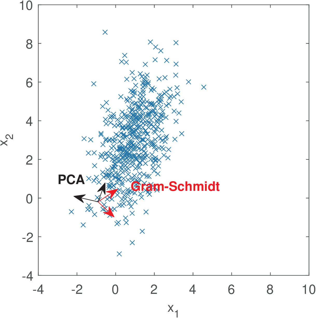
The utility of PCA for representing signals will be illustrated by an example with data draw from a bidimensional Gaussian $f_{{\mathbf{\text{X}}}_1,{\mathbf{\text{X}}}_2}(x_1,x_2)$ with mean $\widehat{\mu }={(1,3)}^T$ and covariance matrix $\mathbf{\text{C}}=\left[\begin{array}{cc}\hfill 1\hfill & \hfill 0.9\hfill \\ \hfill \hfill \\ \hfill \hfill \\ \hfill 0.9\hfill & \hfill 4\hfill \end{array}\right]$. Figure A.4 provides a scatter plot of the data and the basis functions obtained via PCA and, for comparison purposes, Gram-Schmidt orthonormalization. It can be seen that PCA aligns the basis with the directions where the variance is larger. The solution obtained with Gram-Schmidt depends on the first vector and the only guarantee is that the basis functions are orthonormal.

As already indicated, the basis functions of a orthonormal basis can be organized as the columns of a matrix $\mathbf{\text{A}}$. Examples will be provided in the sequel where $\mathbf{\text{A}}$ stores the basis obtained with PCA or the Gram-Schmidt procedure. At this point it is interesting to adopt the same convention used in most textbooks: instead of Eq. (2.1), the input and output vectors are assumed to be related by $\mathbf{\text{x}}=\mathbf{\text{A}}\mathbf{\text{y}}$. In other words, it is the inverse of $\mathbf{\text{A}}$ that transforms $\mathbf{\text{x}}$ into $\mathbf{\text{y}}$: $\mathbf{\text{y}}={\mathbf{\text{A}}}^{-1}\mathbf{\text{x}}$. This is convenient because $\mathbf{\text{y}}$ will be interpreted as storing the transform coefficients of the linear combination of basis functions (columns of $\mathbf{\text{A}}$) that leads to $\mathbf{\text{x}}$.

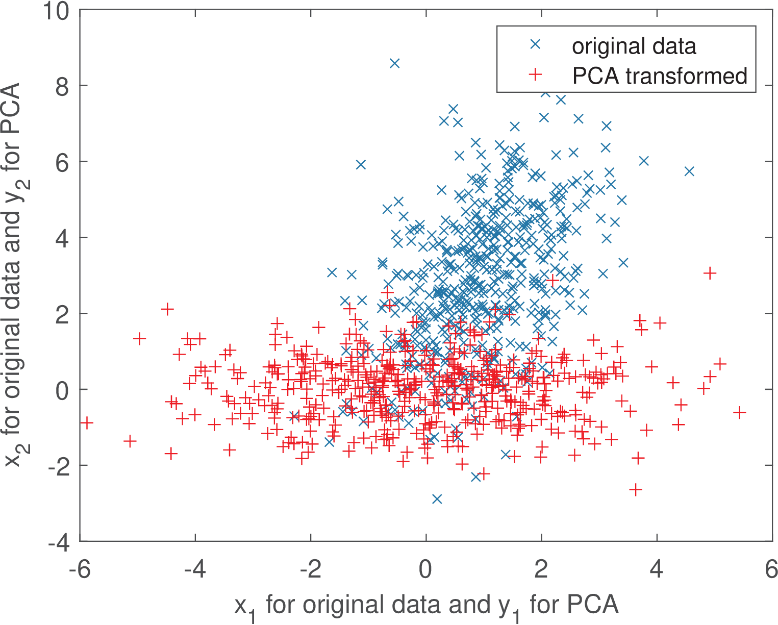
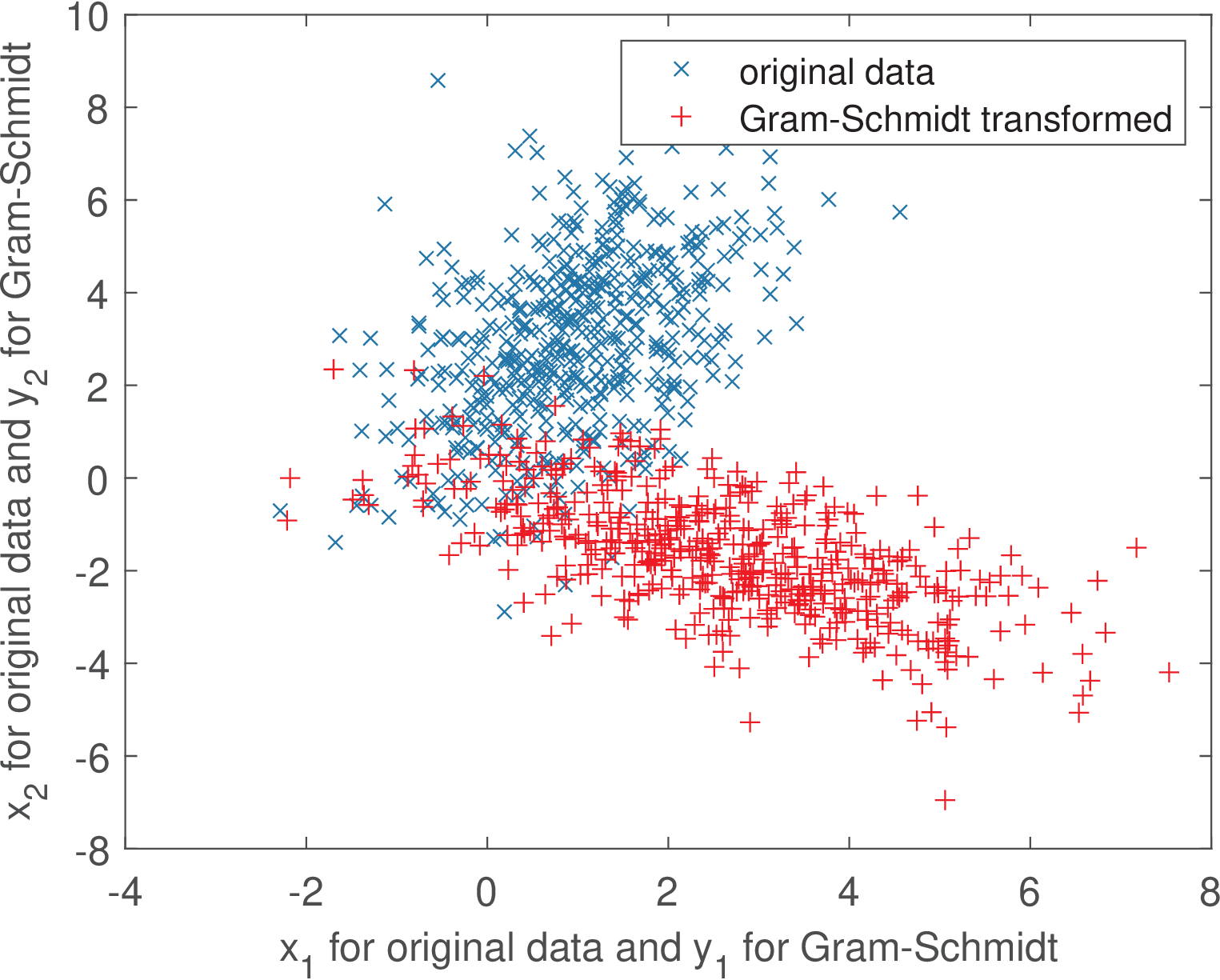
It is possible now to observe the interesting effect of transforming input vectors using PCA and Gram-Schmidt. Using the same input data that generated Figure A.4, Figure A.5 and Figure A.6 show the scatter plots of $\mathbf{\text{y}}$ obtained by $\mathbf{\text{y}}={\mathbf{\text{A}}}^{-1}\mathbf{\text{x}}$, where $\mathbf{\text{A}}$ represents the basis from PCA and Gram-Schmidt, respectively.

Comparing Figure A.5 and Figure A.6 clearly shows that PCA does a better job in extracting the correlation between the two dimensions of the input data. In the Gram-Schmidt case, the figure shows a negative correlation between the coefficients $y_1$ and $y_2$. This is an example of a feature that may be useful. In summary, some linear transforms will be designed such that the basis functions have specified properties while others will focus on properties of the coefficients.