A.14  Linear Algebra

A.14.1  Inner products and norms

In general, a norm is a function $f$ (also denoted as $\text{∥⋅∥}$) that takes a vector $\mathbf{\text{x}}$ and outputs a non-negative real number $y\in {ℝ}_{+}$. The norm $y$ is often interpreted as the distance between $\mathbf{\text{x}}$ and the adopted origin. A norm can be defined for any real or complex vector space, and the vector $\mathbf{\text{x}}$ will belong to this adopted vector space. For example, assuming the Euclidean space and a vector $\mathbf{\text{x}}=[x_1,x_2,\dots ,x_D]$ with real-valued elements, the so-called L2 norm is denoted as $\parallel \mathbf{\text{x}}{\parallel }_2=\sqrt{x_1^2+x_2^2+\dots +x_D^2}$.

Another useful norm is the Manhattan norm $\parallel \mathbf{\text{x}}{\parallel }_1=|x_1|+|x_2|+\dots +|x_D|$, also known as the L1 norm, which correspond to the sum of the absolute values of the elements in vector $\mathbf{\text{x}}$.

A third common norm is the maximum norm $\parallel \mathbf{\text{x}}{\parallel }_{\infty }=\text{max}<!--\; FUNCTION\; APPLICATION\; -->\{|x_1|,|x_2|,\text{…}<!--\; FUNCTION\; APPLICATION\; -->,|x_D|\}$, also known as the infinity norm or Chebyshev norm, which measures the maximum distance along any dimension of the vector. For example, the maximum norm of $\mathbf{\text{x}}=[-3,10,-20]$ is $\parallel \mathbf{\text{x}}{\parallel }_{\infty }=20$.

To be a valid norm, the function $\text{∥⋅∥}$ needs to have some fundamental properties: a) $\parallel \mathbf{\text{x}}\parallel \ge 0$; b) if $\parallel \mathbf{\text{x}}\parallel =0$ then $\mathbf{\text{x}}$ is the zero vector; c) $\parallel \alpha \mathbf{\text{x}}\parallel =|\alpha |\parallel \mathbf{\text{x}}\parallel$ and d) (triangle inequality) $\parallel \mathbf{\text{x}}+\mathbf{\text{y}}\parallel \le \parallel \mathbf{\text{x}}\parallel +\parallel \mathbf{\text{y}}\parallel$.

The inner product in a $K$-dimensional space with complex-valued vectors is:

See Table 2.2 for alternative definitions of inner products.

When $\mathbf{\text{a}}=\mathbf{\text{b}}$, Eq. (A.32) can be written as

An inner product $⟨\mathbf{\text{a}},\mathbf{\text{b}}⟩$ can also be written as a multiplication of two vectors

where in this case both are assumed to be column vectors (row vectors would suggest $\mathbf{\text{a}}{\mathbf{\text{b}}}^H$).

In case a vector $\mathbf{\text{b}}=\mathbf{\text{A}}\mathbf{\text{a}}$ is obtained via multiplication by a unitary matrix $\mathbf{\text{A}}$, Eq. (A.33) and Eq. (A.34) lead to

because ${\mathbf{\text{A}}}^H\mathbf{\text{A}}=\mathbf{\text{I}}$, which indicates that the unitary $\mathbf{\text{A}}$ does not alter the norm of the input vector.

A.14.2  Projection of a vector using inner product

To explore the properties and advantages of linear transforms, it is useful to study the vector projection (or simply projection) of a vector onto another one.

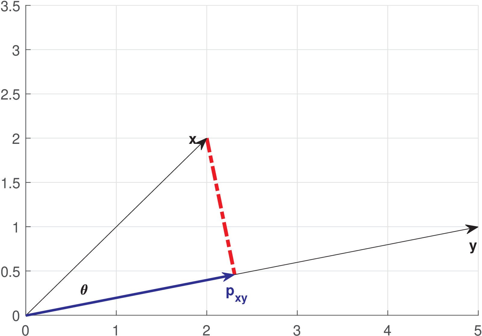
Using ${ℝ}^2$ for simplicity, note that the projection ${\mathbf{\text{p}}}_{\mathit{xy}}$ of a vector $\mathbf{\text{x}}$ in another vector $\mathbf{\text{y}}$ is obtained by choosing the point along the direction of $\mathbf{\text{y}}$ that has the minimum distance to $\mathbf{\text{x}}$. This line is perpendicular to $\mathbf{\text{y}}$, as indicated in Figure A.2. Using the Pythagorean theorem and assuming that $0\le 𝜃\le \pi ∕2$, the norm $\parallel {\mathbf{\text{p}}}_{\mathit{xy}}\parallel$ of the projection can be written as $\parallel {\mathbf{\text{p}}}_{\mathit{xy}}\parallel =\parallel \mathbf{\text{x}}\parallel \text{cos}<!--\; FUNCTION\; APPLICATION\; -->(𝜃)$. If $\pi ∕2<𝜃\le \pi$, $\parallel {\mathbf{\text{p}}}_{\mathit{xy}}\parallel =\parallel \mathbf{\text{x}}\parallel \text{cos}<!--\; FUNCTION\; APPLICATION\; -->(\pi -𝜃)=-\parallel \mathbf{\text{x}}\parallel \text{cos}<!--\; FUNCTION\; APPLICATION\; -->(𝜃)$. Hence, in general,

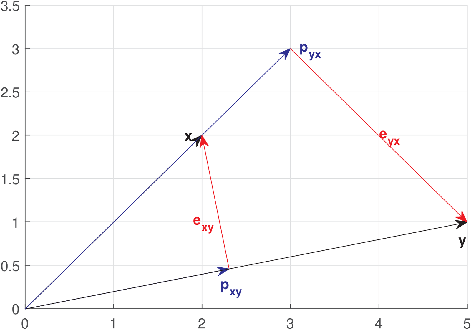
For a given norm $\parallel \mathbf{\text{y}}\parallel$, the larger the inner product, the larger the norm of the projection. The same is valid for ${\mathbf{\text{p}}}_{\mathit{yx}}$ as depicted in Figure A.3:

Any vector $\mathbf{\text{z}}$ can be written as its norm $\parallel \mathbf{\text{z}}\parallel$ multiplied by a unity norm vector $\frac{\mathbf{\text{z}}}{\parallel \mathbf{\text{z}}\parallel }$ that indicates its direction. Note that the vector ${\mathbf{\text{p}}}_{\mathit{yx}}$ is in the same or the opposite direction of $\mathbf{\text{x}}$, which can be specified by the unity norm vector $\mathrm{\text{sign}}(\text{cos}<!--\; FUNCTION\; APPLICATION\; -->(𝜃))\frac{\mathbf{\text{x}}}{\parallel \mathbf{\text{x}}\parallel }$. Hence, one has

where $\frac{⟨\mathbf{\text{x}},\mathbf{\text{y}}⟩}{||\mathbf{\text{x}}|{|}^2}$ is a scaling factor that can be negative but does not change the direction of $\mathbf{\text{x}}$. Similarly, the projection ${\mathbf{\text{p}}}_{\mathit{xy}}$ of $\mathbf{\text{x}}$ onto $\mathbf{\text{y}}$ is given by

Note that if the vector $\mathbf{\text{y}}$ has unitary norm, the absolute value of the inner product $⟨\mathbf{\text{x}},\mathbf{\text{y}}⟩$ coincides with the norm $\parallel {\mathbf{\text{p}}}_{\mathit{xy}}\parallel$. These expressions are valid for other vector spaces, such as ${ℝ}^n$, $n>2$.

Using geometry to interpret a projection vector is very useful. When one projects $\mathbf{\text{x}}$ in $\mathbf{\text{y}}$, the result ${\mathbf{\text{p}}}_{\mathit{xy}}$ is the “best” representation (in the minimum distance sense, or least-square sense) of $\mathbf{\text{x}}$ that $\mathbf{\text{y}}$ alone can provide. The error vector ${\mathbf{\text{e}}}_{\mathit{xy}}=\mathbf{\text{x}}-{\mathbf{\text{p}}}_{\mathit{xy}}$ is orthogonal to $\mathbf{\text{y}}$ (and, consequently, to ${\mathbf{\text{p}}}_{\mathit{xy}}$), i. e., $⟨{\mathbf{\text{e}}}_{\mathit{xy}},\mathbf{\text{y}}⟩=0$. The vector ${\mathbf{\text{e}}}_{\mathit{xy}}$ represents what should be added to ${\mathbf{\text{p}}}_{\mathit{xy}}$ in order to completely represent $\mathbf{\text{x}}$, and the orthogonality $⟨{\mathbf{\text{e}}}_{\mathit{xy}},\mathbf{\text{y}}⟩=0$ indicates that $\mathbf{\text{y}}$ cannot contribute any further.

Figure A.3 completes the example. It was obtained using the following Matlab/Octave script.¹ The example assumes $\mathbf{\text{x}}=[2,2]$ and $\mathbf{\text{y}}=[5,1]$, having an angle $𝜃$ of approximately 33.7 degrees between them.

1x=[2,2]; %define a vector x 
2y=[5,1]; %define a vector y 
3magx=sqrt(sum(x.*x))%magnitude of x 
4magy=sqrt(sum(y.*y))%magnitude of y 
5innerprod=sum(x.*y) %<x,y>=||x|| ||y|| cos(theta) 
6theta=acos(innerprod / (magx*magy)) %angle between x and y 
7%obs: could use acosd to have angle in degrees 
8disp(['Angle is ' num2str(180*theta/pi) ' degrees']); 
9%check if inverting direction is needed: 
10invertDirection=1; if theta>pi/2 invertDirection=-1; end 
11%find the projection of x over y (called p_xy) and p_yx 
12mag_p_xy = magx*abs(cos(theta)) %magnitude of p_xy 
13%directions: obtained as y normalized by magy, x by magx 
14y_unitary=y/magy; %normalize y by magy to get unitary vec. 
15p_xy = mag_p_xy * y_unitary* invertDirection %p_xy 
16mag_p_yx = magy*abs(cos(theta)); %magnitude of p_yx 
17x_unitary=x/magx; %normalize x by magx to get unitary vec. 
18p_yx = mag_p_yx * x_unitary* invertDirection %p_yx 
19%test orthogonality of error vectors: 
20error_xy = x - p_xy; %we know: p_xy + error_xy = x 
21sum(error_xy.*y) %this inner product should be zero 
22error_yx = y - p_yx; %we know: p_yx + error_yx = y 
23sum(error_yx.*x) %this inner product should be zero
  

The concept of projections via inner products will be extensively used in our discussion about transforms. For example, the coefficients of a Fourier series of a signal $x(t)$ correspond to the normalized projections of $x(t)$ on the corresponding basis functions. A large value for the norm of a projection indicates that the given basis function provides a good contribution in the task of representing $x(t)$.

Chapter 2 discusses block transforms and relies on orthogonal functions. Hence, it is useful to discuss why orthogonality is important.

A.14.3  Orthogonal basis allows inner products to transform signals

Assume the existence of a set of orthogonal vectors composing the basis of a vector space. For example, in ${ℝ}^2$, a convenient basis is the standard, composed by $\overline{i}=[1,0]$ and $\overline{j}=[0,1]$. The inner product $⟨\overline{i},\overline{j}⟩=0$ indicates that these two vectors are orthogonal. The orthogonality property simplifies the following analysis task: given any vector $\mathbf{\text{x}}$, the coefficients $\alpha$ and $\beta$ of the linear combination $\mathbf{\text{x}}=\alpha \overline{i}+\beta \overline{j}$, can be easily found by using the dot products $\alpha =⟨\mathbf{\text{x}},\overline{i}⟩$ and $\beta =⟨\mathbf{\text{x}},\overline{j}⟩$. The following theorem proves this important result.

Example A.1. Obtaining the coefficients of a linear combination of basis functions. A simple example can illustrate the analysis procedure: the coefficients of $\mathbf{\text{x}}=4\overline{i}+8\overline{j}$ are $\alpha =4$ and $\beta =8$ by inspection, but they could be calculated as $\alpha =⟨\mathbf{\text{x}},\overline{i}⟩=⟨[4,8],[1,0]⟩=4$ and $\beta =⟨\mathbf{\text{x}},\overline{j}⟩=⟨[4,8],[0,1]⟩=8$. Note that the zeros in these basis vectors make the calculation overly simple. Another example may be more useful to highlight orthogonality and the following alternative basis set is assumed: $\overline{i}=[0.5,0.866]$ and $\overline{j}=[0.866,-0.5]$. Let $\mathbf{\text{x}}=3\overline{i}+2\overline{j}=[3.232,1.5980]$. Given $\mathbf{\text{x}}$, the task is again to find the coefficients such that $\mathbf{\text{x}}=\alpha \overline{i}+\beta \overline{j}$. Due to the orthonormality of $\overline{i}$ and $\overline{j}$, one can for example obtain $\alpha =⟨\mathbf{\text{x}},\overline{i}⟩=⟨[3.232,1.5980],[0.5,0.866]⟩=3$. These computations can be done in Matlab/Octave as follows.

1i=[0.5,0.866], j=[0.866 -0.5] %two orthonormal vectors 
2x=3*i+2*j %create an arbitrary vector x to be analyzed 
3alpha=sum(x.*i), beta=sum(x.*j) %find inner products

In contrast, let us modify the previous example, adopting a non orthogonal basis. Assume that $\overline{i}=[1,1]$ and $\overline{j}=[0,1]$ (note that $⟨\overline{i},\overline{j}⟩=1$, hence the vectors are not orthogonal). Let $\mathbf{\text{x}}=3\overline{i}+2\overline{j}=[3,5]$. In this case, $⟨\mathbf{\text{x}},\overline{i}⟩=8$ and $⟨\mathbf{\text{x}},\overline{j}⟩=5$, which do not coincide with the coefficients $\alpha =3$ and $\beta =2$. How could the coefficients be properly recovered in this case? An alternative is to write the problem as a set of linear equations, organize it in matrix notation and find the coefficients by inverting the matrix. In Matlab/Octave:

1i=transpose([1,1]), j=transpose([0,1]) %non-orthogonal 
2x=3*i+2*j %create an arbitrary vector x to be analyzed 
3A=[i j]; %organize basis vectors as a matrix 
4temp=inv(A)*x; alpha=temp(1), beta=temp(2) %coefficients
  

In summary, the analysis procedure for many linear transforms (such as Fourier, Z, etc.) obtain the coefficients via an inner product, and the procedure can be interpreted as calculating the projection of $\mathbf{\text{x}}$ onto basis $\overline{i}$ (eventually scaled by the norm of $\overline{i}$).   $\text{□}$

This discussion leads to the conclusion that a basis with orthogonal vectors significantly simplifies the task: in this case, the analysis procedure can be done via inner products. This applies when the basis vectors do not have unitary-norm, but in this case a normalization by their norms is needed. Orthogonal basis vectors are a property of all block transforms discussed in this text.

A.14.4  Moore-Penrose pseudoinverse

Pseudoinverses² are generalizations of the inverse matrix and are useful when the given matrix does not have an inverse (for example, when the matrix is not square or full rank).

The Moore-Penrose pseudoinverse has several interesting properties and is adequate to least square problems. It provides the minimum-norm least squares solution $\mathbf{\text{z}}=\mathbf{\text{X}}\mathbf{\text{b}}$ to the problem of finding a vector $\mathbf{\text{z}}$ that minimizes the error vector norm $||\mathbf{\text{X}}\mathbf{\text{z}}-\mathbf{\text{b}}||$. Assuming $\mathbf{\text{X}}$ is an $m\times n$ matrix, the pseudoinverse provides the solution for a set of overdetermined or underdetermined equations if $m>n$ or $m<n$, respectively.

Two properties of a Moore-Penrose pseudoinverse ${\mathbf{\text{X}}}^{+}$ are

and

With $r$ being the rank of $\mathbf{\text{X}}$, then:

• if $m=n$ and $r=m=n$, the pseudoinverse ${\mathbf{\text{X}}}^{+}={\mathbf{\text{X}}}^{-1}$ is equivalent to the usual inverse;

• if $m>n$ (overdetermined) and, besides, $r=n$ (the columns of $\mathbf{\text{X}}$ are linearly independent), ${\mathbf{\text{X}}}^H\mathbf{\text{X}}$ is invertible and using Eq. (A.37) the pseudoinverse is given by

  $${\mathbf{\text{X}}}^{+}={\left({\mathbf{\text{X}}}^H\mathbf{\text{X}}\right)}^{-1}{\mathbf{\text{X}}}^H;$$

  (A.39)

• if $n>m$ (underdetermined) and $r=m$ (the rows of $\mathbf{\text{X}}$ are linearly independent), $\mathbf{\text{X}}{\mathbf{\text{X}}}^H$ is invertible and using Eq. (A.38) leads to

  $${\mathbf{\text{X}}}^{+}={\mathbf{\text{X}}}^H{\left(\mathbf{\text{X}}{\mathbf{\text{X}}}^H\right)}^{-1}.$$

  (A.40)

Whenever available, instead of Eq. (A.39) or Eq. (A.40) that requires linear independence, one should use a robust method to obtain ${\mathbf{\text{X}}}^{+}$ such as the pinv function in Matlab/Octave, which adopts a SVD decomposition to calculate ${\mathbf{\text{X}}}^{+}$. Listing A.3 illustrates such calculations and the convenience of relying on pinv when the independence of rows or columns is not guaranteed.

1test=3; %choose the case below 
2switch test 
3    case 1 %m>n (overdetermined/tall) and linearly indepen. columns 
4        X=[1 2 3; -4+1j -5+1j -6+1j;1 0 0;0 1 0]; %4 x 3 
5    case 2 %n>m (underdetermined/fat) and linearly independent rows 
6        X=[1 2 3; -4+1j -5+1j -6+1j]; %2 x 3 
7    case 3 %neither rows nor columns of X are linearly independent 
8        %rows X(2,:)=2*X(1,:) and columns X(:,4)=3*X(:,1) 
9        X=[1 2 3 3; 2 4 6 6; -4+1j -5+1j -6+1j -12+3*1j]; %3 x 4 
10end 
11Xp_svd = pinv(X) %pseudoinverse via SVD decomposition 
12Xp_over = inv(X'*X)*X' %valid when columns are linearly independent 
13Xp_under = X'*inv(X*X') %valid when rows are linearly independent 
14rank(X'*X) %X'*X is square but may not be full rank 
15rank(X*X') %X*X' is square but may not be full rank 
16Xhermitian=X'*X*pinv(X) %equal to X' (this property is always valid) 
17Xhermitian2=pinv(X)*X*X' %equal to X' (the property itself is valid) 
18maxError_over=max(abs(Xp_svd(:)-Xp_over(:))) %error for overdetermin. 
19maxError_under=max(abs(Xp_svd(:)-Xp_under(:))) %for underdetermined