1.6  Signal Categorization

This section discusses important categories of signals and their distinctive properties.

1.6.1  Even and odd signals

A signal $x[n]$ is called even if $x[n]=x[-n]$, and odd if $x[n]=-x[-n]$. The definitions are also valid for a continuous-time signal and, in general, for any function $f(x)$. An even function $f(x)$ has the property that $f(x)=f(-x)$, while an odd function has the property that $f(x)=-f(-x)$. For instance, the cosine is an even function while the sine is an odd function.

Interestingly, any function can be decomposed into even $f_e(x)$ and odd $f_o(x)$ parts, such that $f(x)=f_e(x)+f_o(x)$. The two component parts can be obtained as

Similarly, any signal $x[n]$ (or $x(t)$) can be obtained as the sum of an even $x_e[n]$ and odd $x_o[n]$ parcels, which can be found as follows:

and

respectively, such that $x[n]=x_e[n]+x_o[n]$.

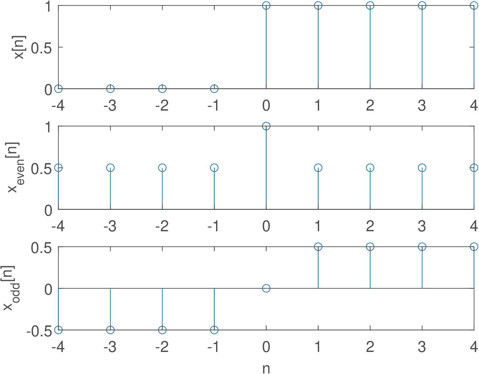
For example, assume the unit step function $x(t)=u(t)$. Its even and odd parts are $x_e(t)=0.5,\forall <!--\; FUNCTION\; APPLICATION\; -->t$ and $x_o(t)=0.5u(t)-0.5u(-t)$, respectively.

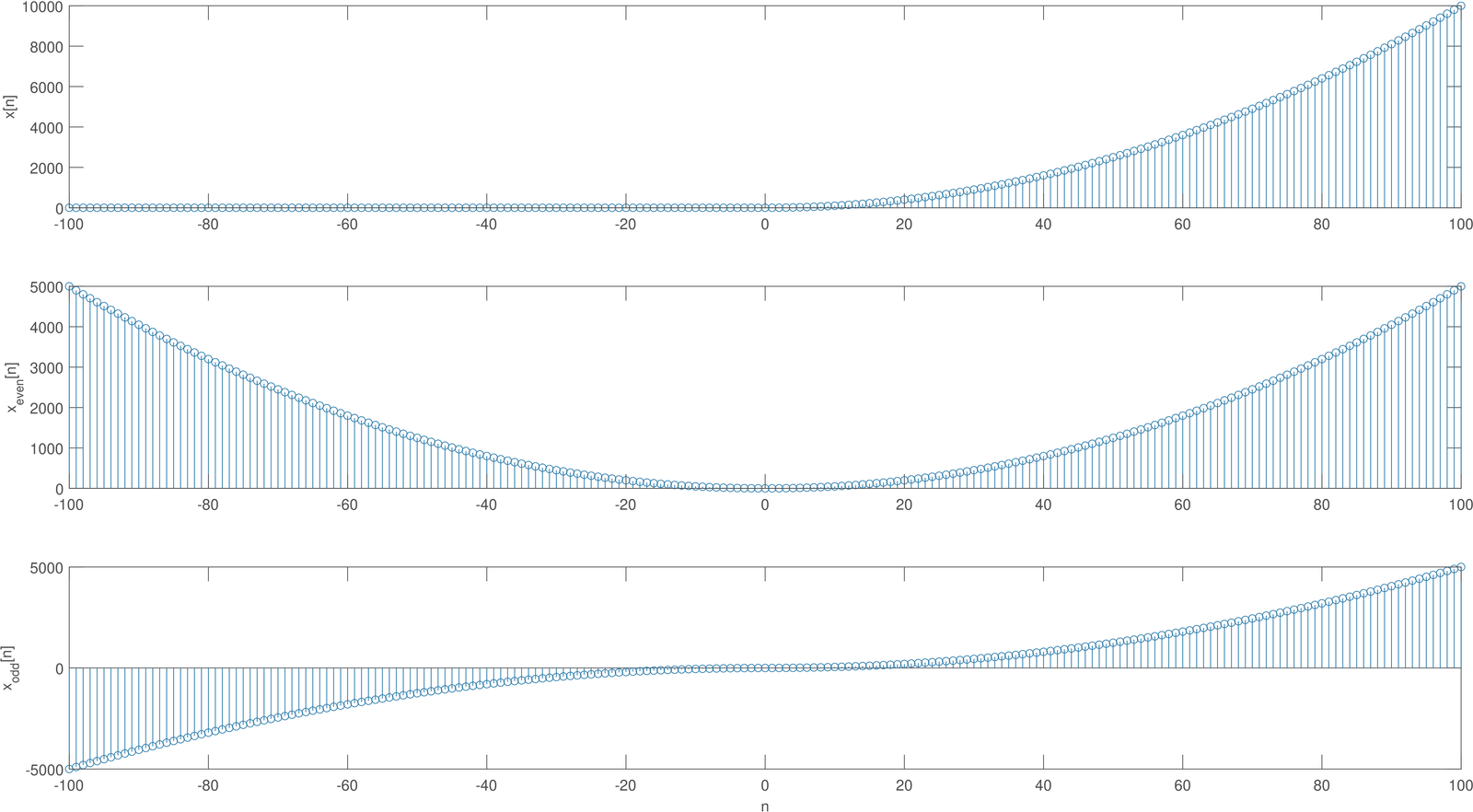
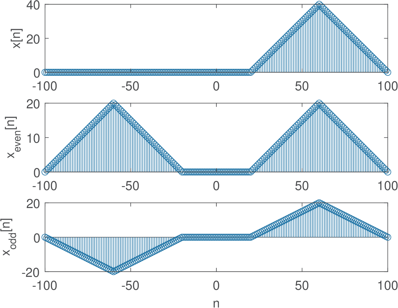
The function ak_getEvenOddParts.m can be used to obtain the even and odd components of arbitrary finite-duration sequences. Three examples are provided in Figure 1.16, Figure 1.17 and Figure 1.18.

1.6.2  Random signals and their generation

Random signals are important to represent noise or other non-deterministic signals. Discrete-time random signals of finite duration can be represented by vectors in which the elements are outcomes of random variables (see Appendix A.19). For example, assuming all elements of [2, 0, 2, 3, 3, 2, 3] are outcomes of the same random variable $X$, one can calculate the average $𝔼[X]\approx 2.14$, the standard deviation $\sigma \approx 1.07$ and other statistical moments of $X$.

Alternatively, a vector with random samples may correspond to a realization of a discrete-time random process (see Appendix A.20).

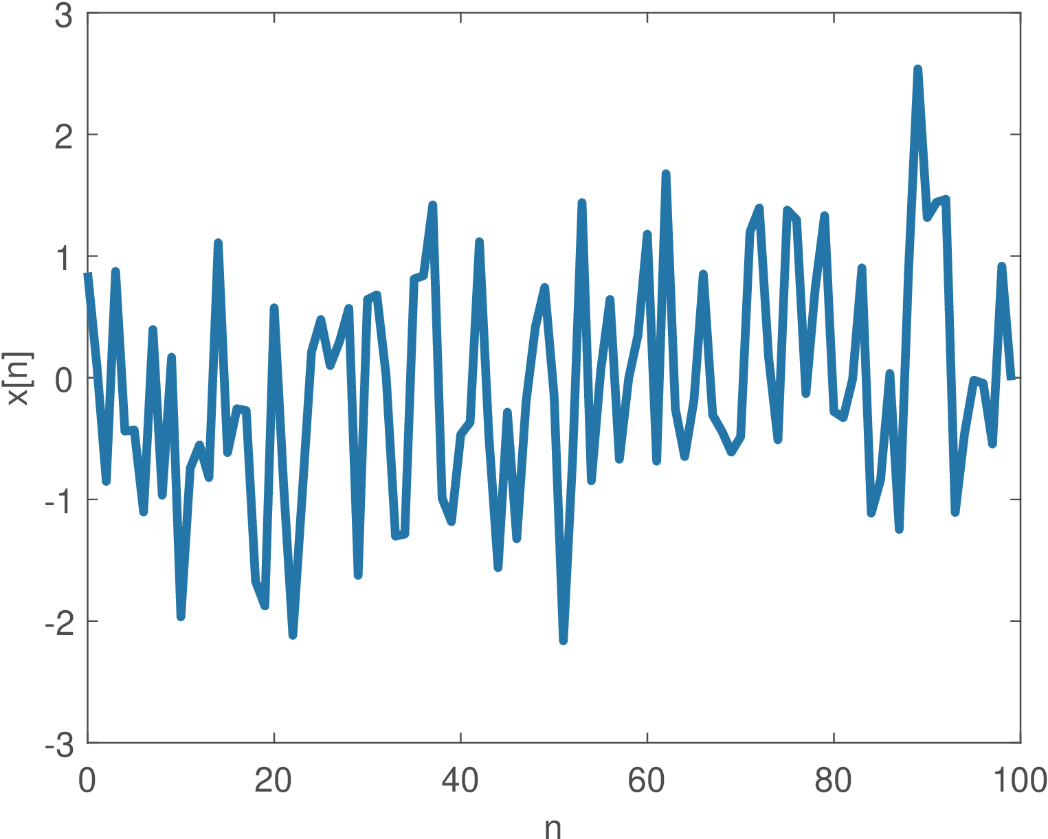
Example 1.11. Random Gaussian signals: generation, waveform and histogram. It is easy to generate random signals in Matlab/Octave. For example, the command x=randn(1,100) generates 100 samples distributed according to a standard Gaussian (zero-mean and unity-variance) distribution $N(0,1)$, where the notation $N(\mu ,{\sigma }^2)$ assumes the second argument is the variance ${\sigma }^2$, not the standard deviation $\sigma$. These signals can be visualized as a time-series,⁸ such as in Figure 1.19.

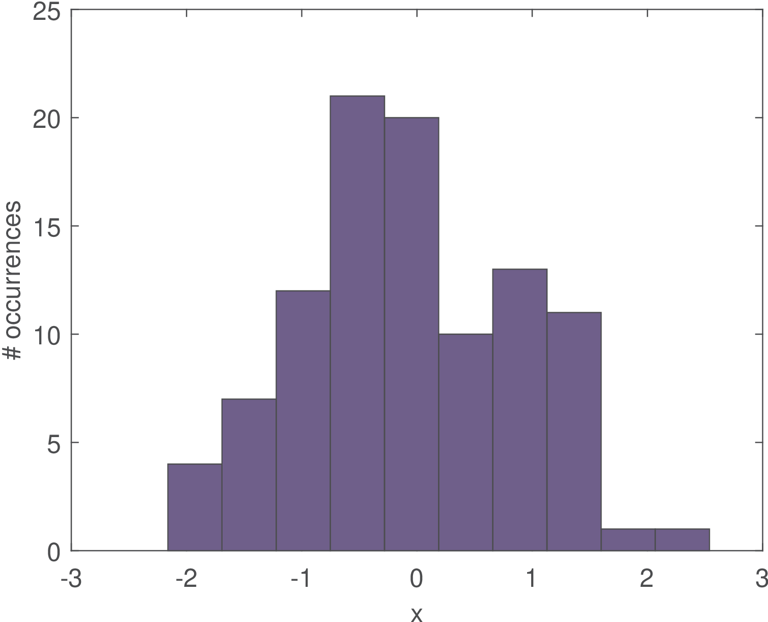
The time-domain visualization can be complemented by plotting the probability distribution of the random signal. Figure 1.20 illustrates the histogram of the signal depicted in Figure 1.19. The histogram is calculated by dividing the dynamic range in bins and counting the number of samples that belong to each bin. Figure 1.20 was obtained by using $B=10$ bins (the default).

Figure 1.21 can help in case the reader is not familiar with the notion of a histogram bin. An example of Matlab/Octave commands that would lead to these $B=3$ bins are: x=[1, 3.1, 2.6, 4]; [counts,centers] = hist(x,3).

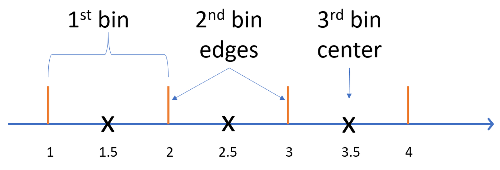
Histograms can also be easily generated with Python. For instance, using numpy one can create a histogram with the $B=3$ bins in Figure 1.21 with the commands:

1import numpy as np 
2x=np.array([1, 3.1, 2.6, 4]) 
3hist, bin_edges = np.histogram(x,3)

While Matlab/Octave returns the bin centers, Python’s numpy returns the bin edges. In both languages, the first and last edge values (1 and 4, in the example of Figure 1.21) correspond to the minimum $x_{\mathrm{\text{min}}}$ and maximum $x_{\mathrm{\text{max}}}$ values of the input signal. The bin width is given by

which leads to $\mathrm{\text{bin\_width}}=1$ in Figure 1.21.   $\text{□}$

The histogram indicates the number of occurrences of the input data within the ranges (or bins) indicated in its abscissa. The histogram is also very useful to estimate a probability mass function (PMF) and probability density function (PDF) from available data, which are used for discrete and continuous random variables, respectively.

Example 1.12. Using a normalized histogram as an estimate of the probability mass function. Even when the elements of the input vector x are real values, the histogram calculation “quantizes” these input values into only $B$ values, which represent the ranges of the histogram bins. In other words, the bin centers can be seen as the result of a quantization process. Besides peforming this “quantization”, the histogram also indicates the number of occurrences of these $B$ values in x.

The $B$ center bins of a histogram can be interpreted as the possible distinct values of a discrete random variable. Therefore, normalizing the histogram by the total number $N$ of samples provides an estimate of the PMF of this discrete random variable.

For instance, suppose a vector x with N=100 elements. Calculating the histogram and dividing the number of occurrences by N provides an estimate of the PMF of x. In Matlab/Octave, after obtaining the histogram with [occurrences, bin_centers]=hist(x), the PMF can be estimated using stem(bin_centers, occurrences/N).    $\text{□}$

Normalizing the histogram by the total number $N$ of samples provides an estimate of the PMF of a discrete random variable, with values represented by centers of the histogram bins. When this result is further normalized by the bin width, an estimate of the PDF is obtained, as discussed in the next example.

Example 1.13. Using a normalized histogram as an estimate of the probability density function. Sometimes we know the input data x is composed of realizations of a continuous random variable with a known PDF. When the task is to superimpose a PDF estimated from data to the actual PDF, one needs to properly normalize the histogram (see Appendix A.13).

The function ak_normalize_histogram.m can be used to estimate a PDF from a histogram and was used to obtain Figure 1.22 according to the commands in Listing 1.7.

1B=10; %number of bins 
2x=randn(1,100); %random numbers ~ G(0,1) 
3[n2,x2]=ak_normalize_histogram(x,B);%PDF via normalized histogram 
4a=-3:0.1:3; %use range of [-3std, 3std] around the mean 
5plot(x2,n2,'o-',a,normpdf(a),'x-') %estimate vs. theoretical PDF
  

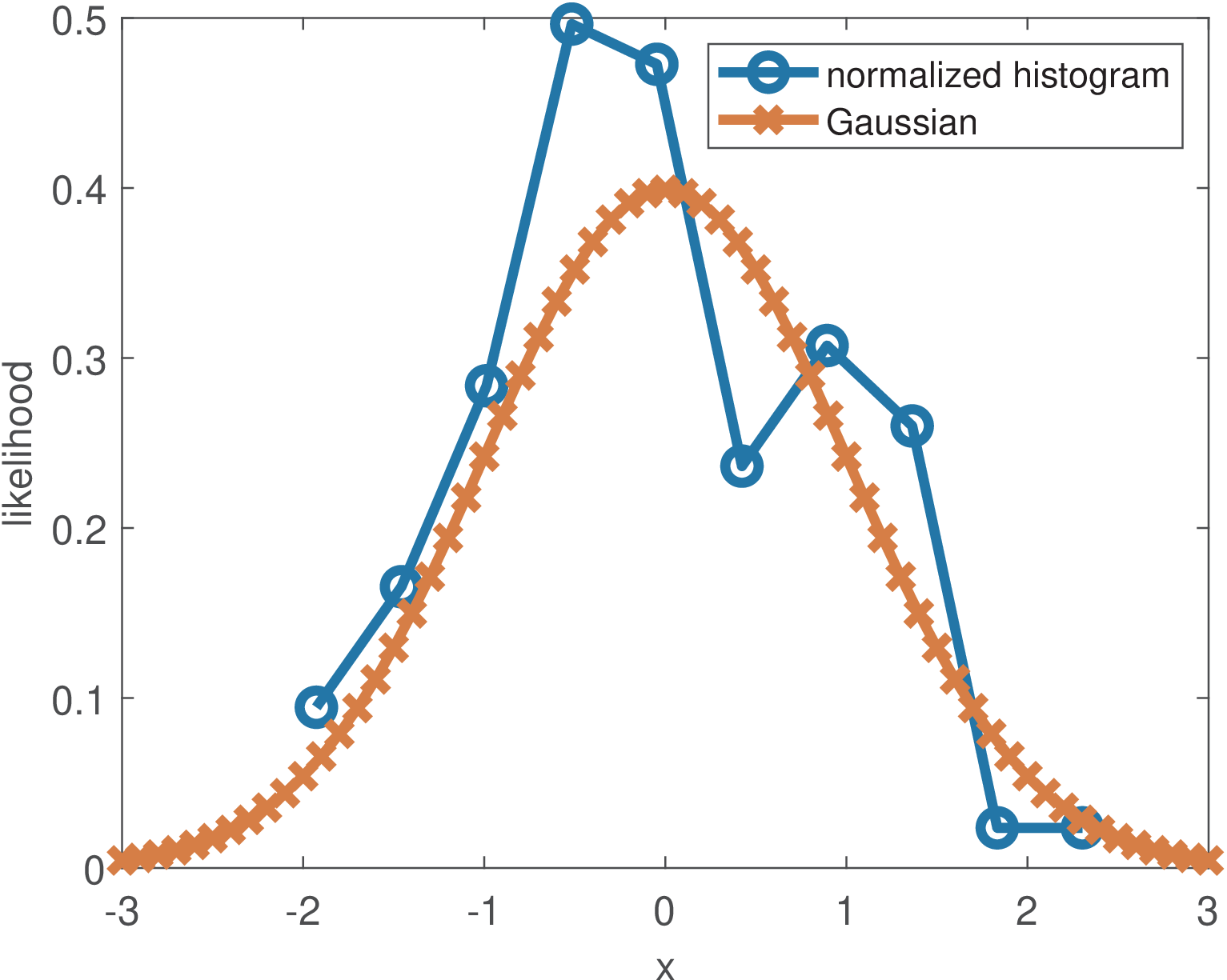
Figure 1.22 indicates that 100 samples and 10 bins provide only a crude estimation.    $\text{□}$

Example 1.14. Changing the mean and variance of a random variable. Assume a random variable $X$ has a mean $\eta =𝔼[X]$ and $N$ of its realizations compose a vector x. If one wants to create a new random variable $Y$ with $𝔼[Y]=\eta +3$, this can be done with $Y=X+3$, or using the realizations: y=x+3. This is valid for any constant value $\kappa$.

To prove it, observe that the expected value is a linear operator (see, Appendix A.19.3), such that when $Y=X+\kappa$, one has

Similarly, if the variance of $X$ is ${\sigma }_x^2$, a random variable $Y=\sqrt{\kappa }X$ has variance ${\sigma }_y^2=\kappa {\sigma }_x^2$. The proof is based on Eq. (A.67) and linearity:

Take now the particular example of the function randn in Matlab/Octave, which generates realizations of a random variable $X$ that is distributed according to the normalized Gaussian $N(0,1)$. Based on Eq. (1.16) and Eq. (1.17), if one creates a new random variable $Y=\sigma X+\eta$, the mean and variance of $Y$ are $\eta$ and ${\sigma }^2$, respectively.

Considering Matlab/Octave, the command x=sqrt(newVariance)*randn(1,N)+newMean provides Gaussians with arbitrary mean and variance.

Listing 1.8 was used to generate the samples of $N(4,0.09)$ and illustrates how to draw samples from a Gaussian with any given mean and variance from calls to a random number generator that outputs samples from a standard Gaussian $N(0,1)$.

1newMean=4; %new mean 
2newVariance=0.09; %new variance 
3N=10000; %number of random samples 
4x=sqrt(newVariance)*randn(1,N)+newMean;
  

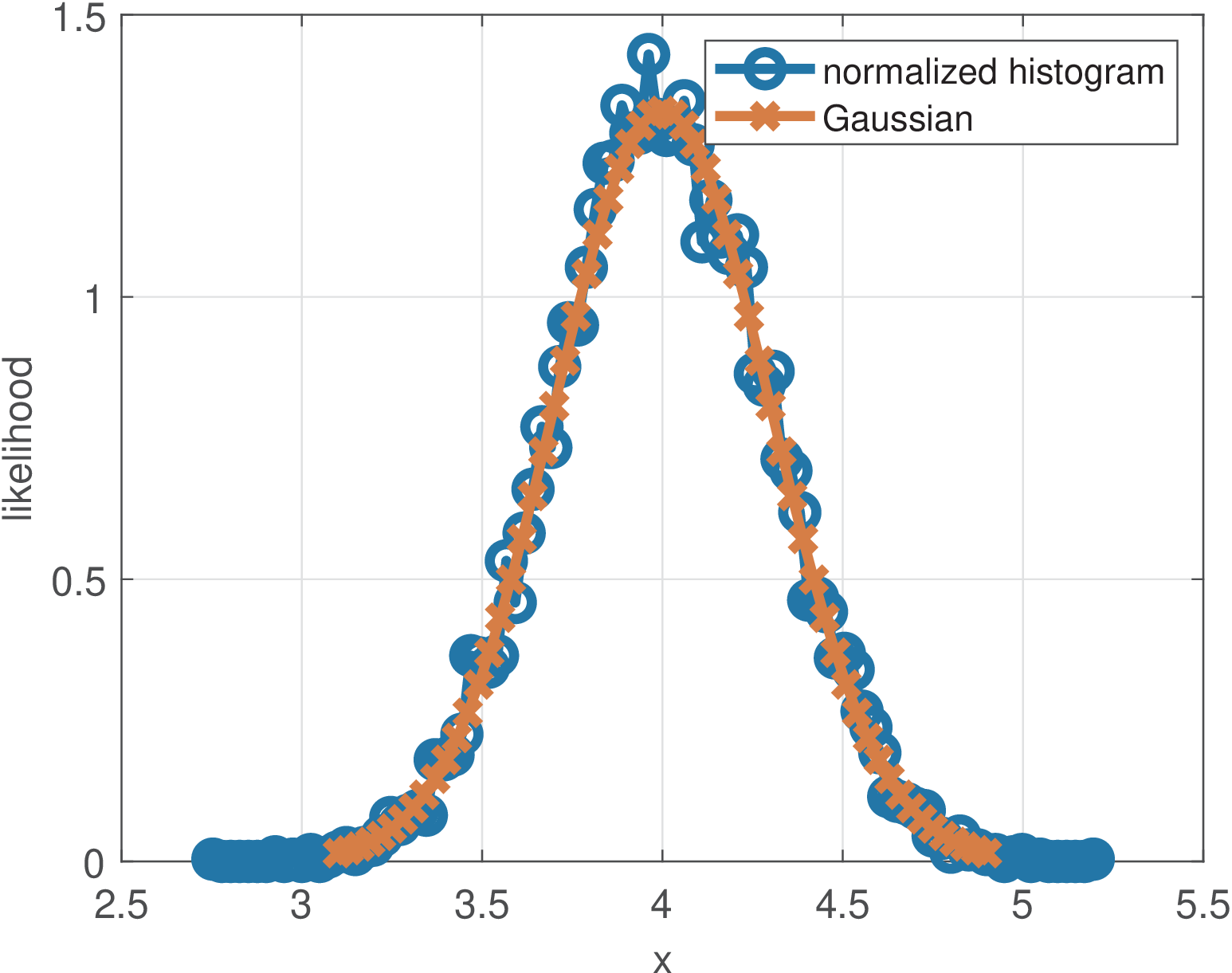
Figure 1.23 was obtained by using 10 thousand samples from a Gaussian $N(4,0.09)$ and using 100 bins for the histogram. Now the Gaussian estimation is relatively good when compared to the one depicted in Figure 1.22.

It should be noted that the normalized histogram of a continuous PDF indicates likelihood, not probability. The likelihood function is the PDF viewed as a function of the parameters. Therefore, it is possible to have values larger than one in the ordinate, such as in Figure 1.23.    $\text{□}$

While the previous example assumed a Gaussian PDF, the next one deals with a uniform PDF.

Example 1.15. Calculating and changing the mean and variance of a uniform probability density function. A random variable $X$ distributed according to a uniform PDF with support $[a,b]$ (range from $a$ to $b$ of values that have non-zero likelihood) has a mean given by

and variance:

Eq. (1.19) can be proved observing that the uniform PDF $f_X(x)$ is a constant $1∕(b-a)$ over the range $[a,b]$ and zero otherwise. Hence, using Eq. (A.69) with the function $g(X)=g({(X-\mu )}^2)$ leads to

where $S=b-a$ is the PDF support.

When using the random number generator rand for uniformly distributed samples, one should notice that the dynamic range is $[0,1]$, i. e., $a=0$ and $b=1$. Hence, Eq. (1.18) indicates the mean is 0.5 and the variance given by Eq. (1.19) is $S^2∕12=1∕12\approx 0.0833$.

Drawing from rand, it is possible to generate N samples uniformly distributed in an arbitrary range $[a,b]$ with the command x = a + (b-a) * rand(N,1).   $\text{□}$

1.6.3  Periodic and aperiodic signals

Periodicity in continuous-time

A signal $x(t)$ (same discussion applies to $x[n]$) is periodic if a given segment of $x(t)$ is eternally repeated, such that $x(t)=x(t+T)$ for some $T>0$, where $T$ is called the period. For example, if $T=10$ seconds and $x(t)=x(t+10)$, for all values of $t$.

In the example of $T=10$, it is easy to check that $x(t)=x(t+20)$, $x(t)=x(t+30)$ and so on. In other words, a signal with period $T$ is also periodic in $2T,3T,\dots$. The fundamental period $T_0$ is the smallest value of $T$ for which $x(t)=x(t+T_0)$. Note that the definition imposes $T_0>0$ and a constant signal $x(t)=\kappa$ is not considered periodic.

Example 1.16. Using the LCM and GCD for a periodic signal composed by commensurate frequencies. Two frequencies $f_1$ and $f_2$ are called commensurate if their ratio $f_1∕f_2$ can be written as a rational number $m∕n$, where $m,n$ are non-zero integers. Instead of frequencies, one can use their associated time periods.

Assume a signal $x(t)={\sum <!--\; FUNCTION\; APPLICATION\; -->}_{i=1}^N{x}_i(t)$ is composed by the sum of $N$ periodic components $x_i(t)$, each one with period $T_i$ and frequency $f_i=1∕T_i$. The set of frequencies $\{f_i\}$ is commensurate if all pairs are commensurate. In this case, the fundamental period $T_0$ of $x(t)$ can be found using the least common multiple (LCM) of the periods $\{T_i\}$ while the fundamental frequency $F_0=1∕T_0$ can be found using the greatest common divisor (GCD) of the frequencies $\{f_i\}$. Assuming both LCM and GCD are defined only for integer numbers, it may be needed to extract a common factor and later reintroduce it. A numerical example helps: let $x(t)=\text{cos}<!--\; FUNCTION\; APPLICATION\; -->(2\pi f_{1}t)+\text{cos}<!--\; FUNCTION\; APPLICATION\; -->(2\pi f_{2}t+\pi ∕2)+\text{sin}<!--\; FUNCTION\; APPLICATION\; -->(2\pi f_{3}t)$ be composed by sinusoids with frequencies $f_1=5∕2$, $f_2=1∕6$ and $f_3=1∕8$ Hz, which corresponds to periods $T_1=0.4$, $T_2=6$ and $T_3=8$ seconds, respectively. To find the LCM, one may need to multiply all periods by 10 and then calculate that $\mathrm{\text{LCM}}(4,60,80)=240$. Dividing this result by the factor 10 leads to $T_0=24$ s. This LCM could be obtained in Matlab/Octave with lcm(lcm(4,60),80) given that this function is limited to accepting only two input arguments.    $\text{□}$

Periodicity of a generic discrete-time signal

A discrete-time signal is periodic if $x[n]=x[n+N_0]$ for some integer $N_0>0$. Similar to the continuous-time case, the value $N_0$ is called the fundamental period if it corresponds to the minimum number of samples in which the amplitudes repeat.

Periodicity of discrete-time sinusoids

One important thing is that the discrete-time counterpart of some periodic analog signals may be non-periodic. The next paragraphs discuss the periodicity of discrete-time sinusoids such as $\text{cos}<!--\; FUNCTION\; APPLICATION\; -->((\pi ∕4)n)$, $\text{sin}<!--\; FUNCTION\; APPLICATION\; -->(3n)$ and $e^{\mathit{\pi n}}$. For example the signal $x(t)=\text{cos}<!--\; FUNCTION\; APPLICATION\; -->(3t)$ is periodic with period $T=2\pi ∕3$ s. However, the discrete-time signal $x[n]=\text{cos}<!--\; FUNCTION\; APPLICATION\; -->(3n)$ is non-periodic.

A discrete-time sinusoid such as $x[n]=A\text{cos}<!--\; FUNCTION\; APPLICATION\; -->(\mathrm{\Omega }n+\varphi )$ is periodic only if $\mathrm{\Omega }∕(2\pi )$ is a ratio $m∕N_0$ of two integers $m$ and $N_0$ as proved below.⁹ One can write:

If the parcel $\mathrm{\Omega }{N}_0$ in previous expression is a multiple of $2\pi$, then $x[n+N_0]=x[n],\forall <!--\; FUNCTION\; APPLICATION\; -->n$. Hence, periodicity requires $\mathrm{\Omega }{N}_0=2\mathit{\pi m}$, which leads to the condition

for a discrete-time sinusoid to be periodic.

Example 1.17. Checking the periodicity of discrete-time sinusoids. For example, $x[n]=\text{cos}<!--\; FUNCTION\; APPLICATION\; -->(3n)$ is non-periodic because $\mathrm{\Omega }=3$ and $3∕(2\pi )$ cannot be written as a ratio of two integers. In contrast, $x[n]=\text{cos}<!--\; FUNCTION\; APPLICATION\; -->((2\pi ∕8)n+0.2)$ is periodic with period $N_0=8$ ($m=1$ in this case). The signal $x[n]=\text{cos}<!--\; FUNCTION\; APPLICATION\; -->(7\mathit{\pi n})$ is periodic because $\mathrm{\Omega }=7\pi$ and $\mathrm{\Omega }∕(2\pi )=7∕2$, with $m=7$ and $N_0=2$.    $\text{□}$

If $m∕N_0$ in Eq. (1.21) is an irreducible fraction, then $N_0$ is the fundamental period. Otherwise, $N_0$ may be a multiple of the fundamental period.

Example 1.18. Finding the fundamental period requires reducing the fraction $m∕N_0$. For instance, the signal $x[n]=\text{cos}<!--\; FUNCTION\; APPLICATION\; -->((12\pi ∕28)n)$ is periodic because $\mathrm{\Omega }=(12\pi ∕28)$ and $\mathrm{\Omega }∕(2\pi )=6∕28$, with $m=6$ and $N_0=28$. However, if one is interested on the fundamental period, it is necessary to reduce the fraction $6∕28$ to $3∕14$, and obtain the fundamental period as $N_0=14$ samples.   $\text{□}$

In summary, when contrasting continuous and discrete-time sinusoids, to find the period $T$ of a continuous-time cosine $\text{cos}<!--\; FUNCTION\; APPLICATION\; -->(\mathit{\omega t}+\varphi )$, one can obtain the term $\omega$ that multiplies $t$ and calculate

which is given in seconds if $\omega$ is in rad/s. Hence, a continuous-time sinusoid is always periodic. But a discrete-time cosine $\text{cos}<!--\; FUNCTION\; APPLICATION\; -->(\mathrm{\Omega }n+\varphi )$ may be quasi periodic (i. e., not periodic). If someone tries to simply calculate $N_0=\frac{2\pi }{\mathrm{\Omega }}$, it may end up with a non-integer period. The condition for periodicity is to be able to write $2\pi ∕\mathrm{\Omega }$ as a ratio of integers, i. e.

where $N_0$ is the period in samples. After turning an $N_0∕$ an irreducible fraction, $N_0$ is the fundamental period.

Example 1.19. Meaning of $m$ when determining the fundamental period. To understand the role of $m$, consider the signal $\text{cos}<!--\; FUNCTION\; APPLICATION\; -->((3\pi ∕17)n)$. In this case, $\frac{2\pi }{\mathrm{\Omega }}=34∕3$ cannot be the period because it is not an integer. However, if one allows for $m=3$ times the number of samples specified by $\frac{2\pi }{\mathrm{\Omega }}$, the result is the integer period $N_0=m\frac{2\pi }{\mathrm{\Omega }}=34$ samples. See Application 1.6 for a discussion on finding $m$ and $N_0$ using Matlab/Octave.

Sometimes, it is misleading to guess the period of a discrete-time cosine or sine via the observation of its graph. Figure 1.24 depicts the graph of $x[n]=\text{sin}<!--\; FUNCTION\; APPLICATION\; -->(0.2n)$ and was obtained with the following code:

1M=100, w=0.2; %%num of samples and angular freq. (rad) 
2n=0:M-1; %generate abscissa 
3xn=sin(w*n); stem(n,xn); %generate and plot a sinusoid

In this case, the signal seems to have a period around 31 samples at a first glance (because $2\pi ∕\mathrm{\Omega }\approx 31.4$). But, for example, $x[n]$ will never be 0 at the beginning of a cycle for a value of $n$ other than $n=0$. Therefore, in spite of resembling a periodic signal, the angular frequency $\mathrm{\Omega }$ is such that $2\pi ∕\mathrm{\Omega }=10\pi$ is a irrational number and a cycle of numbers will never repeat. In this case, the signal is called almost or quasi periodic.¹⁰

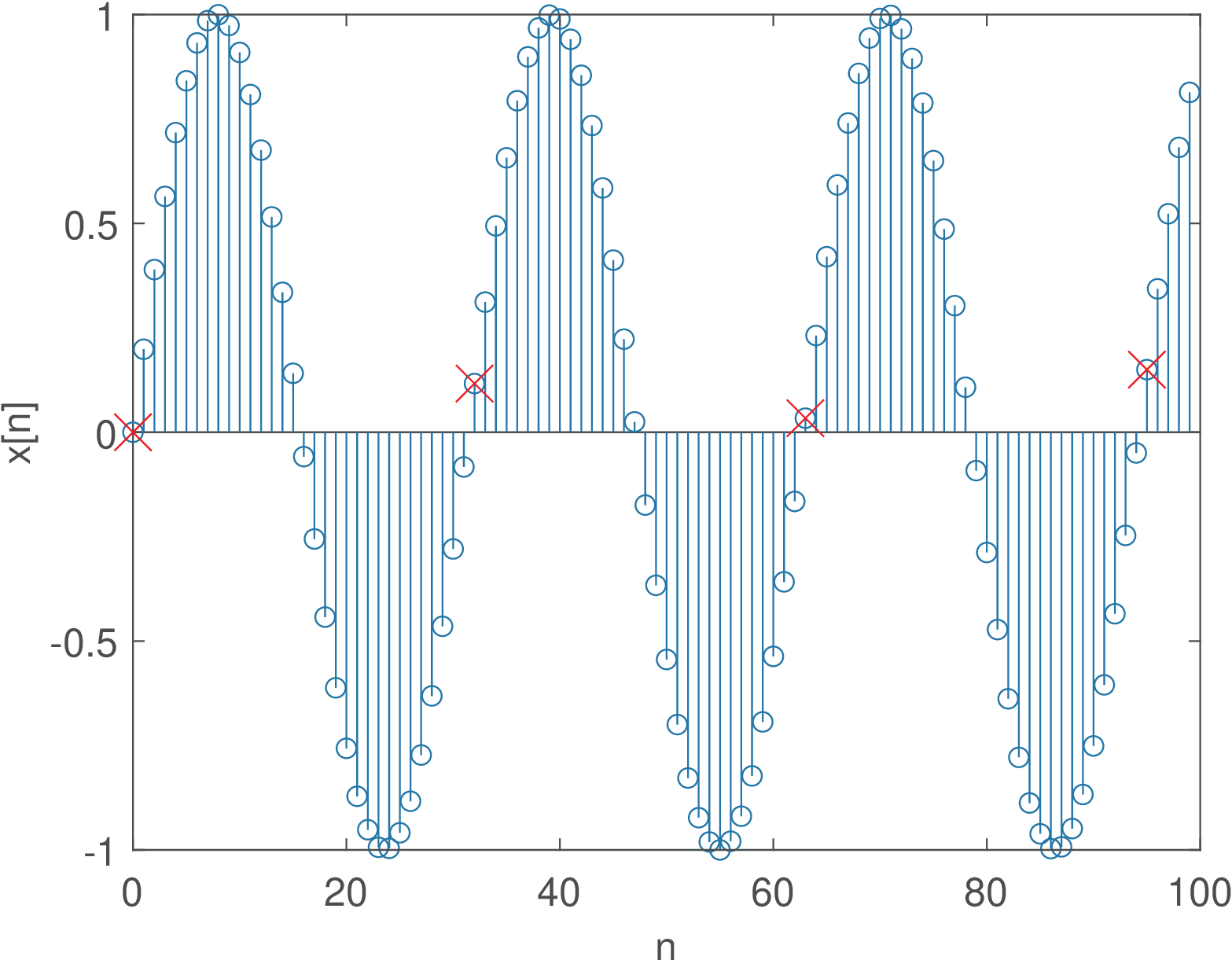
It is useful to visualize a discrete-time sinusoid that is periodic with $m>1$. Figure 1.25 depicts the graph of $x[n]=\text{sin}<!--\; FUNCTION\; APPLICATION\; -->((3\pi ∕17)n)$ and illustrates the repetition of $m=3$ sine envelopes within a period of $N_0=34$ samples.

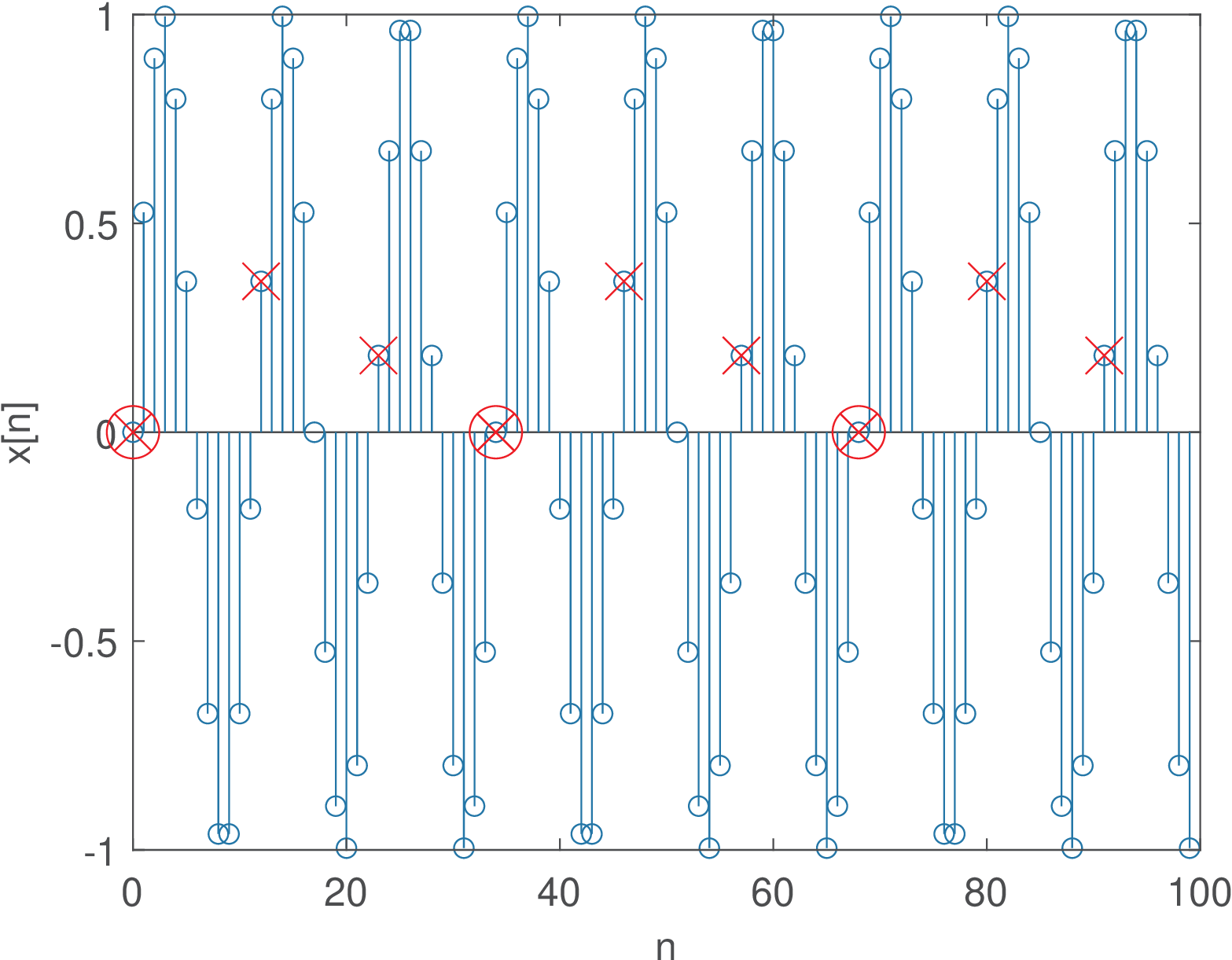
Figure 1.24 and Figure 1.25 illustrate how to distinguish strictly periodic sinusoids from quasi periodic, and help interpreting $m$ in Eq. (1.21).   $\text{□}$

1.6.4  Power and energy signals

It is important to understand the concepts of power $P$ and energy $E$ of a signal. One reason is that, in some cases, the equation to be used for a specific analysis (autocorrelation, for example) differs depending if $P$ or $E$ are not finite. This section assumes continuous-time but the concepts are also valid for discrete-time signals.

If $E$ is the energy dissipated by a signal during a time interval $\mathrm{\Delta }t$, the average power along $\mathrm{\Delta }t$ is

If $p(t)=|x(t){|}^2$ is the instantaneous power of $x(t)$, $E$ can be calculated as

If the interval $\mathrm{\Delta }t$ is not specified, it is implicitly assumed (by default) the whole time axis $]-\infty ,\infty [$ and

In this case, $P$ is defined as the limit

Note that, because the time interval goes to infinite (denominator), $P$ is zero unless the energy $E$ (numerator) also goes to infinite. This situation suggests the definition of power and energy signals, which have finite power and energy, respectively. Their characteristics are summarized in Table 1.3, which also indicates that there is a third category for signals that have neither finite power or energy.

The most common power signals are periodic. In this case, the energy $E_T$ in one period $T$

can be used to easily calculate

because what happens in one period is replicated along the whole time axis.

The most common energy signals have a finite duration, such as $x(t)=t^2[u(t)-u(t-5)]$. Assuming the signals have finite amplitude, their energy in a finite time interval cannot be infinite. Note that infinite duration signals, such as $x(t)=e^{-t}u(t)$, can also have a finite energy in case their amplitude decay over time.

It is assumed throughout this text that the signals are currents $i(t)$ or voltages $v(t)$ over a resistance $R$, such that the instantaneous power is

Besides, to deal with signals $x(t)$ representing both currents and voltages without bothering about the normalization by $R$, it is assumed that $R=1$ ohm. Hence, the instantaneous power is $p(t)=x^2(t)$ for any real $x(t)$ and, more generally, $p(t)=|x(t){|}^2$ in case $x(t)$ is complex-valued.

Throughout the book, unless stated otherwise, $x(t)$ is assumed to be in volts, $p(t)$ and $P$ in watts and $E$ in joules. A dimensional analysis of $p(t)=x^2(t)$ should not be interpreted directly as watts = ${\mathrm{\text{volts}}}^2$, but watts = ${\mathrm{\text{volts}}}^2$/ohm, where the normalization by 1 ohm is implicit. Two examples are provided in the sequel.

Example 1.20. Sinusoid power. Sinusoids and cosines can be represented by $x(t)=A\text{cos}<!--\; FUNCTION\; APPLICATION\; -->({\omega }_{0}t+𝜃)$ and are power signals with average power $P=\frac{A^2}{2}$. The phase $𝜃$ does not influence the power calculation. The proof follows.

The angular frequency is ${\omega }_0=\frac{2\pi }{T}$ rad/s, where $T$ is the period in seconds.

Using the identity ${\text{cos}<!--\; FUNCTION\; APPLICATION\; -->}^{2}a=\frac{1}{2}(\text{cos}<!--\; FUNCTION\; APPLICATION\; -->(2a)+1)$ (see Appendix):

The first parcel of the integral is zero, independent of $2𝜃$ because $T$ corresponds exactly to two periods of the cosine with angular frequency $2{\omega }_0$, while the second parcel is $T$. The average power is

which is a result valid for any sinusoid or cosine. This discussion assumed continuous-time signals, but Eq. (1.24) is also valid for discrete-time sinusoids.    $\text{□}$

Example 1.21. Power of a DC signal. A constant signal $x(t)=K$ (i. e., a DC signal) has power $P=K^2$ because the energy at any interval $\mathrm{\Delta }t$ is $E=K^2\mathrm{\Delta }t$.    $\text{□}$

The root-mean-square (RMS) value $x_{\mathrm{\text{rms}}}$ of any signal $x(t)$ is the DC value that corresponds to the same power $P$ of $x(t)$, i. e., $x_{\mathrm{\text{rms}}}^2=P$ or, equivalently, $x_{\mathrm{\text{rms}}}=\sqrt{P}.$ For example, the RMS value of a cosine $x(t)=A\text{cos}<!--\; FUNCTION\; APPLICATION\; -->({\omega }_{0}t+𝜃)$ is $x_{\mathrm{\text{rms}}}=\frac{A}{\sqrt{2}}$ because a DC signal $y(t)=\frac{A}{\sqrt{2}}$ has the same average power as $x(t)$.

As discussed in Section A.26.4, $\delta (t)$ is a distribution and it is tricky to define the energy or power of a sampled signal, which is the topic of Section 3.5.2.