1.4 Block or Window Processing
Many algorithms segment the signal into blocks of samples and process each block individually. For example, when writing Matlab/Octave code for DSP, it is tempting to organize the information in a single vector, which is then processed and converted into another vector. This works well when the number of elements in each vector is relatively small. However, many situations require processing billions of samples, and the corresponding long vectors would eventually not fit in memory. In these cases, the best strategy is to write DSP code using block processing, also called window processing and frame-based processing.
1.4.1 Block processing without overlapping
When processing a discrete-time “infinite” duration signal in blocks (also called window or frames), is iteratively segmented and represented by finite dimensional vectors with elements each. Assuming that is a right-sided signal ( corresponds to the first non-zero sample, to the second and so on), the first block is formed by the samples
In general, the -th block is represented by the column vector
|
| (1.9) |
To avoid too many indexes, the dependence on will be omitted hereafter.
Example 1.10. Segmenting a signal into blocks. Suppose the task is to segment a very long signal into blocks and then calculate the power of each block. Listing 1.7 illustrates how to perform this task in Matlab/Octave.
1S=10000; %some arbitrary number of samples
2x=rand(1,S); %create some very very long vector
3N=50; %number of samples per frame (or block)
4M=floor(S/N); %number of blocks, floor may discard last block samples
5powerPerBlock=zeros(M,1); %pre-allocate space
6for m=0:M-1 %following the book convention
7    beginIndex = m*N+1; %index of the m-th block start
8    endIndex = beginIndex+N-1; %m-th block end index
9    xm=x(beginIndex:endIndex) %the samples of m-th block
10    powerPerBlock(m+1)=mean(abs(xm).^2); %estimate power of block xm
11end
12clf; subplot(211); plot(x); subplot(212); plot(powerPerBlock) %plot
Note that Eq. (1.9) assumes the first index is 0, which is adopted in Python, C, Java and other languages. However, in Matlab/Octave the first index is 1 and this required using beginIndex = m*N+1 instead of beginIndex = m*N as in Eq. (1.9).
The reader is invited to use a speech signal instead of the random signal and observe how the signal power varies over time, comparing it for vowels and consonants.
1.4.2 Advanced: Block processing with overlapped windows
The next paragraphs discuss an alternative to deal with observation windows containing samples (or observations). It is assumed that for each window, it is desired to obtain a single estimate. For instance, one can use windows with samples to estimate the average signal power within that window. The goal is to extract more information from the available collection of samples and alleviate the noise and blocking effects. Two strategies to improve block processing are overlapping windows and multiplying the block of samples by a function with support of samples and that goes to zero at its endpoints. The function is called window and is discussed in Section 4.3. Here, we will solely rely on overlapping windows, as illustrated in Figure 1.18.
To specify the extraction of overlapping windows, besides the length , one needs to define the shift in samples. When the window shift (also called stride in deep learning) is , neighboring windows share samples. Figure 1.18 provides an example in which and . As also indicated in this figure, non-overlapping windows are obtained with
|
| (1.10) |
With , for each new input sample, there is a new observation window and consecutive windows share samples. For example, in Figure 1.18, when sample comes, the observation window slides to the right and encompasses to . When comes, the window covers to , and so on. In this case, because there is a new estimate for each new sample, the estimator’s output rate is the same as its input rate despite the value of . Another application of overlapping window is in estimating the spectogram, as explained in Section 4.11.1.

When dealing with block processing, it is sometimes useful to adopt a windowed indexing in which represents the -th sample of the -th window, as depicted in Figure 1.18.
When there are available samples, the number of windows with samples and shifted by samples that can be extracted is given by
|
| (1.11) |
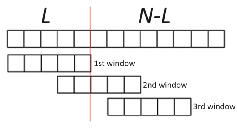
where all values , and are greater than zero, and (otherwise there is not a single window). For example, if we have samples, with windows of samples and shifted by , the result is windows.
To prove Eq. (1.11), it must be taken into account that of the input samples, we need to make one valid window and hence the summation of 1. As depicted in Figure 1.19, for the remaining samples, , each extra valid window requires samples. The floor function eliminates incomplete windows. This is illustrated in Figure 1.19, where the red line separates, at the left, samples for the first window, and the remaining samples are enough for two extra valid windows (each one requires samples). In this example, the last two of the samples are not used in any window.
