1.13  Applications

Some applications of the main results in this chapter are discussed in this section.

Application 1.1. PC sound board quantizer. Given a system with an ADC, typically one has to know beforehand or conduct measurements to obtain the quantizer step size $\mathrm{\Delta }$. This is the case when using a personal computer (PC) sound board. For a sound board, the value of $\mathrm{\Delta }$ depends if the signal was acquired using the microphone input or the line-in input of the sound board. The microphone interface is designed for signals with peak value of $X_{\mathrm{\text{max}}}=10$ to 100 mV while the peak for the line-in is typically 0.2 to 2 V. Note that the voltage ranges of line inputs and microphones vary from card to card. See more details in [ url1pcs]. For the sake of this discussion, one can assume a dynamic range of $[-100,100]$ mV and a ADC of 8 bits per sample, such that $\mathrm{\Delta }=200∕(2^8-1)\approx 0.78$ mV. The following example illustrates how to approximately recover the analog signal for visualization purposes. Assume the digital dynamic range is [0, 255] and the digital samples are $D=[13,126,3,34,254]$. If one simply uses stem(D), there is no information about time and amplitude. Listing 1.25 shows the necessary normalizations to visualize the abscissa in seconds and the ordinate in volts, which in this case corresponds to A=1000*[-89.70, -1.56, -97.50, -73.32, 98.28].

1D=[13 126 3 34 254]; %signal as 8-bits unsigned [0, 255] 
2n=[0:4]; %sample instants in the digital domain 
3Fs=8000; %sampling frequency 
4delta=0.78e-3; %step size in Volts 
5A=(D-128)*delta; %subtract offset=128 and normalize by delta 
6Ts=1/Fs; %sampling interval in seconds 
7time=n*Ts; %normalize abscissa 
8stem(time,A); %compare with stem(n,D) 
9xlabel('time (s)'); ylabel('amplitude (V)');  

Now assume a PC computer with a sound board that uses a 16 bits ADC and supports at its input a dynamic range of $-185$ to $185$ mV. The quantizer is similar to the one depicted in Figure 1.54, but the quantization step should be $\mathrm{\Delta }=2\times 185\times 10^{-3}∕2^{16}\approx 5.6$ $\mu$V. It is assumed here that $\mathrm{\Delta }=5.6$ $\mu$V and the quantizer is uniform from $-2^{15}\mathrm{\Delta }$ to $(2^{15}-1)\mathrm{\Delta }$. In this case, the $M=65,536=2^{16}$ levels are organized as 32,767 positive levels, 32,768 negative levels and one level representing zero. The assumed coding scheme is the offset code of Table 1.8 with 32,768 as the offset. Hence, the smallest value $-2^{15}\mathrm{\Delta }$ is mapped to the 16-bits codeword “0000 0000 0000 0000”, $(-2^{15}+1)\mathrm{\Delta }$ to “0000 0000 0000 0001” and so on, with $(2^{15}-1)\mathrm{\Delta }$ being coded as “1111 1111 1111 1111”.

If at a specific time $t_0$ the ADC input is $x(t_0)=x=0.003$ V, the ADC output is $x_i=536$, which corresponds to $x_q=0.0030016$ V and leads to a quantization error $e=x-x_q\approx -1.6\times 10^{-6}$ V. These results can be obtained in Matlab/Octave with

1delta=5.6e-6, b=16 %define parameters for the quantizer 
2format long %see numbers with many decimals 
3x=3e-3; [xq,xi]=ak_quantizer(x,delta,b), error=x-xq

Based on similar reasoning, calculate the outputs $x_i$ of the quantizer, their respective $x_q$ values and the quantization error for $x\in \{-300,-100,0,20,180\}$ mV.

If you have access to an oscilloscope and a function generator, try to estimate the value of $\mathrm{\Delta }$ of your sound board, paying attention to the fact that some software/hardware combination use automatic gain control (AGC). You probably need to disable AGC to better control the acquisition.

It is not trivial, but if you want to learn more about your sound board, try to evaluate its performance according to the procedure described at [ url1bau].    $\text{□}$

Application 1.2. A simple application of correlation analysis. A company produces three distinct beauty creams: A, B and C. The task is the analysis of correlation in three databases, one for each product. The contents of each database can be represented by two vectors $\mathbf{\text{x}}$ and $\mathbf{\text{y}}$, with 1,000 elements each. Vector $\mathbf{\text{x}}$ informs the age of the consumer and $\mathbf{\text{y}}$ the number of his/her purchases of the respective cream (A, B or C) during one year, respectively. Figure 1.66 depicts scatter plots corresponding to each product.

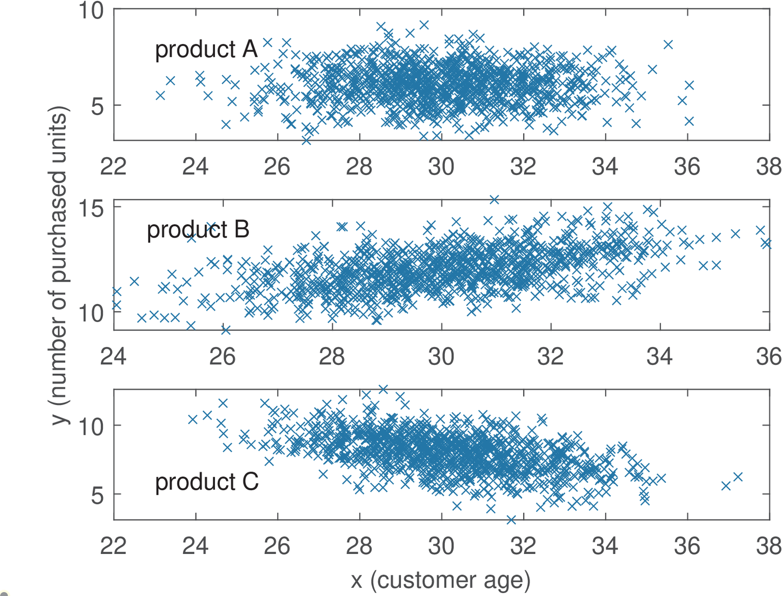
The empirical (the one calculated from the available data) covariance matrices and means were approximately the following: ${\mathbf{\text{C}}}_a=\left[\begin{array}{cc}\hfill 4.08\hfill & \hfill -0.002\hfill \\ \hfill \hfill \\ \hfill \hfill \\ \hfill -0.002\hfill & \hfill 0.98\hfill \end{array}\right]$ and ${\mu }_a=[30.0,6.05]$, ${\mathbf{\text{C}}}_b=\left[\begin{array}{cc}\hfill 4.00\hfill & \hfill 0.99\hfill \\ \hfill \hfill \\ \hfill \hfill \\ \hfill 0.99\hfill & \hfill 1.00\hfill \end{array}\right]$and ${\mu }_b=[30.1,12.0]$, ${\mathbf{\text{C}}}_c=\left[\begin{array}{cc}\hfill 4.16\hfill & \hfill -1.46\hfill \\ \hfill \hfill \\ \hfill \hfill \\ \hfill -1.46\hfill & \hfill 2.02\hfill \end{array}\right]$and ${\mu }_c=[30.13,7.99]$. The correlation coefficients are ${\rho }_a=-0.0011$, ${\rho }_b=0.4924$ and ${\rho }_c=-0.5031$.

The plots and correlation coefficients indicate that when age increases, the sales of product B also increases (positive correlation). In contrast, the negative correlation of ${\rho }_b$ indicates that the sales of product C decreases among older people. The sales of product A seem uncorrelated with age. The script figs_signals_correlationcoeff.m allows to study how the data and figures were created. Your task is to learn how to generate two-dimensional Gaussians with arbitrary covariance matrices.

Note that the correlation analysis was performed observing each product sales individually. You can assume the existence of a unique database, where each entry has four fields: age, sales of A, B and C. What kind of analysis do you foresee? For example, one could try a marketing campaign that combines two product if their sales are correlated. Or even use data mining tools to extract association rules that indicate how to organize the marketing.    $\text{□}$

Application 1.3. Playing with the autocorrelation function of white noise and sinusoids. Using randn in Matlab/Octave, generate a vector corresponding to a realization of a WGN process (see Example 1.56): x=randn(1,1000). Check whether or not it is Gaussian by estimating the FDP (use hist). Plot its autocorrelation with the proper axes. Generate a new signal that is uniformly distributed: y=rand(1,1000)-0.5; and plot the same graphs as for the Gaussian signal. What does it happen with the autocorrelation if you add a DC level (add a constant to x and y)? And what if you multiply by a number (a “gain”)? Generate a cosine T=0.01; t=0:T:10-T; z=cos(2*pi*10*t); of 10 Hz with a sampling frequency of 100 Hz. Take a look at the autocorrelation for lags from $m=-30,\dots ,30$ with [c,lags]=xcorr(z,30,’biased’);plot(lags,c). Compare this last plot with a zoom of the cosine: plot(z(1:30)). Note that they have the same period. In fact, an autocorrelation $R$ of $x$ incorporates all the periodicity that is found in $x$ as indicated by Eq. (1.62). Make sure you can use Eq. (1.62) to predict the plots you obtain with xcorr when the signal is a sinusoid.   $\text{□}$

Application 1.4. Using autocorrelation to estimate the cycle of sunspot activity. The international sunspot number (also known as the Wolfer number) is a quantity that simultaneously measures the number and size of sunspots. A sunspot is a region on the Sun’s surface that is visible as dark spots. The number of sunspots correlates with the intensity of solar radiation: more sunspots means a brighter sun. This number has been collected and tabulated by researchers for around 300 years. They have found that sunspot activity is cyclical and reaches its maximum around every 9.5 to 11 years (in average, 10.4883 years).²⁷ The autocorrelation can provide such estimate as indicated by the script below. Note that we are not interested in $R(0)$, which is always the maximum value of $R(\tau )$. The lag of the largest absolute value of $R(\tau )$ other than $R(0)$ indicates the signal fundamental period. Because theoretically no other value can be larger than $R(0)$, the task of automatically finding the second peak (not the second largest sample), which is the one of interest, is not trivial. The code snippet below simply (not automatically) indicates the position of the second peak for the sunspot data.

1load sunspot.dat; %the data file 
2year=sunspot(:,1); %first column 
3wolfer=sunspot(:,2); %second column 
4%plot(year,wolfer); title('Sunspot Data') %plot raw data 
5x=wolfer-mean(wolfer); %remove mean 
6[R,lag]=xcorr(x); %calculate autocorrelation 
7plot(lag,R); hold on; 
8index=find(lag==11); %we know the 2nd peak is lag=11 
9plot(lag(index),R(index),'r.', 'MarkerSize',25); 
10text(lag(index)+10,R(index),['2nd peak at lag=11']);  

Figure 1.67 shows the graph generated by the companion script figs_signals_correlation.m. It complements the previous code snippet, showing how to extract the second peak automatically (this can be useful in other applications of the ACF). Your task is to study this code and get prepared to work with “pitch” estimation in Application 1.5.

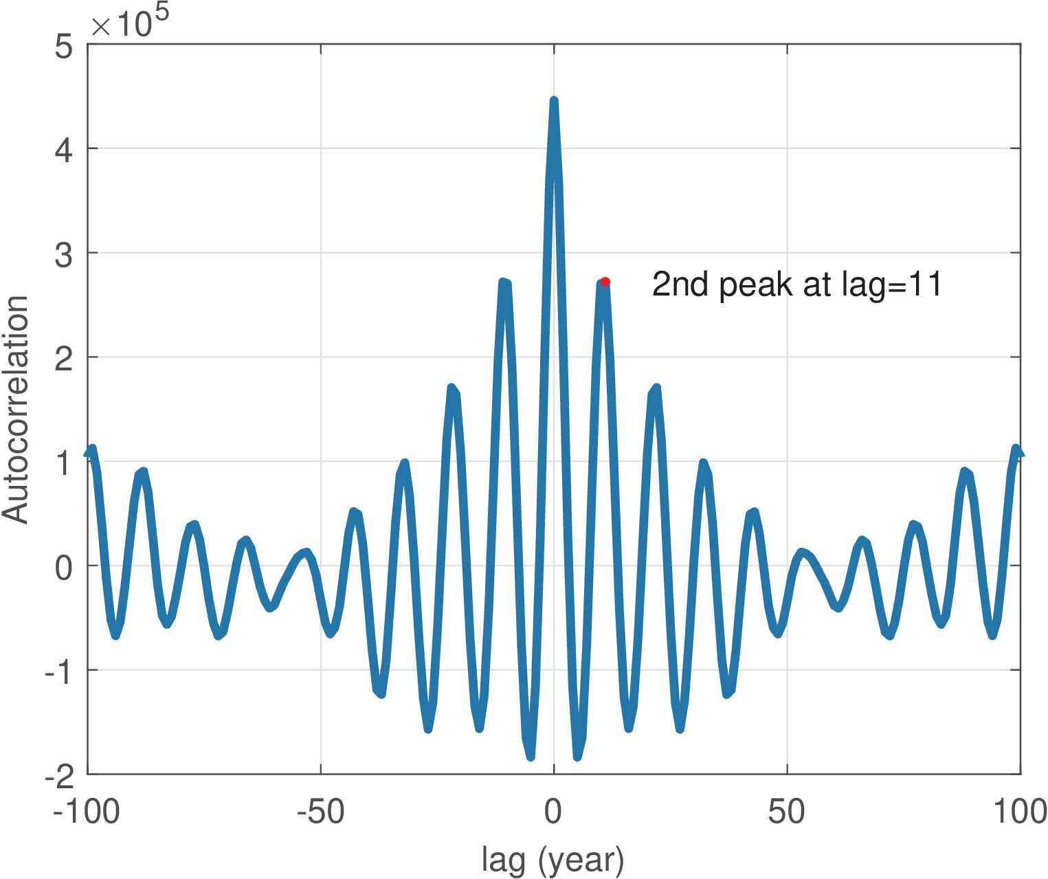
An important aspect of the sunspot task is the interpretation of $R(\tau )$. As discussed, when the autocorrelation has a peak, it is an indication of high similarity, i. e., periodicity. In the sunspot application, the interval between two lags was one year. If the ACF is obtained from a signal sampled at $F_s$ Hz, this interval between lags is the sampling period $T_s=1∕F_s$ and it is relatively easy to normalize the lag axis. The next example illustrates the procedure.    $\text{□}$

Application 1.5. Using autocorrelation to estimate the “pitch”. This application studies a procedure to record speech, estimate the average fundamental frequency $F0$ (also erroneously but commonly called pitch) via autocorrelation and play a sinusoid with a frequency proportional to $F0$.

One can estimate the fundamental frequency of a speech signal by looking for a peak in the delay interval corresponding to the normal pitch range in speech.²⁸ The following script illustrates the procedure.

1Fs=44100; %sampling frequency 
2Ts=1/Fs; %sampling interval 
3minF0Frequency=80; %minimum F0 frequency in Hz 
4maxF0Frequency=300; %minimum F0 frequency in Hz 
5minF0Period = 1/minF0Frequency; %correponding F0 (sec) 
6maxF0Period = 1/maxF0Frequency; %correponding F0 (sec) 
7Nbegin=round(maxF0Period/Ts);%number of lags for max freq. 
8Nend=round(minF0Period/Ts); %number of lags for min freq. 
9if 0 %record sound or test with 300 Hz cosine 
10    r = audiorecorder(Fs, 16, 1);%object audiorecorder 
11    disp('Started recording. Say a vowel a, e, i, o or u') 
12    recordblocking(r,2);%record 2 s and store in object r 
13    disp('finished recording'); 
14    y=double(getaudiodata(r, 'int16'));%get recorded data 
15else %test with a cosine 
16    y=cos(2*pi*300*[0:2*Fs-1]*Ts); %300 Hz, duration 2 secs 
17end 
18subplot(211); plot(Ts*[0:length(y)-1],y); 
19xlabel('time (s)'); ylabel('Signal y(t)') 
20[R,lags]=xcorr(y,Nend,'biased'); %ACF with max lag Nend 
21subplot(212); %autocorrelation with normalized abscissa 
22plot(lags*Ts,R); xlabel('lag (s)'); 
23ylabel('Autocorrelation of y(t)') 
24firstIndex = find(lags==Nbegin); %find index of lag 
25Rpartial = R(firstIndex:end); %just the region of interest 
26[Rmax, relative_index_max]=max(Rpartial); 
27%Rpartial was just part of R, so recalculate the index: 
28index_max = firstIndex - 1 + relative_index_max; 
29lag_max = lags(index_max); %get lag corresponding to index 
30hold on; %show the point: 
31plot(lag_max*Ts,Rmax,'xr','markersize',20); 
32F0 = 1/(lag_max*Ts); %estimated F0 frequency (Hz) 
33fprintf('Rmax=%g lag_max=%g T=%g (s) Freq.=%g Hz\n',... 
34    Rmax,lag_max,lag_max*Ts,F0); 
35t=0:Ts:2; soundsc(cos(2*pi*3*F0*t),Fs); %play freq. 3*F0  

Figure 1.68 was generated using the previous script with the signal $y(t)$ consisting of a cosine of 300 Hz instead of digitized speech (simply change the logical condition of the “if”).

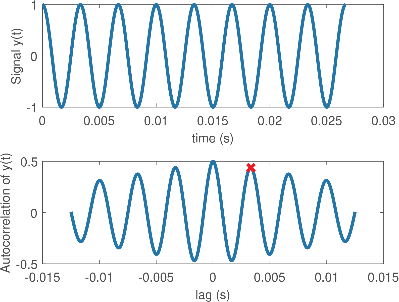
The code outputs the following results:
Rmax=0.49913 lag_max=147 T=0.00333333 (sec) Frequency=300 Hz
Note that the autocorrelation was normalized xcorr(y,Nend,’biased’), which led to $R(0)\approx 0.5$ Watts, coinciding with the sinusoid power $A^2∕2$, where $A=1$ V is the sinusoid amplitude.

As commonly done, in spite of dealing with discrete-time signals, the graphs assume the signals are approximating a continuous-time signal and ACF. Hence, the abscissa is $t$, not $n$.

Some PC sound boards heavily attenuate the signals around 100 Hz. Therefore, the last command multiplies the estimated $F0$ by 3, to provide a more audible tone. Modify the last line of the code to use $F0$ instead of $3F0$ and observe the result of varying F0 with your own voice. Then try to improve the code to create your own F0 estimation algorithm. Find on the Web a Matlab/Octave F0 (or pitch) estimation algorithm to be the baseline (there is one at [ url1pit]) and compare it with your code. Use the same input files for a fair comparison and superimpose the pitch tracks to spectrograms to better compare them. If you enjoy speech processing, try to get familiar with Praat [ url1pra] and similar softwares and compare their F0 estimations with yours.    $\text{□}$

Application 1.6. Using cross-correlation for synchronization of two signals or time-alignment. Assume a discrete-time signal $x[n]$ is transmitted through a communication channel and the receiver obtains a delayed and distorted version $y[n]$. The task is to estimate the delay imposed by the channel. The transmitter does not “stamp” the time when the transmission starts, but uses a predefined preamble sequence $p[n]$ that is known by the receiver. The receiver will then guess the beginning of the transmitted message by searching for the preamble sequence in $y[n]$ via cross-correlation. Before trying an example that pretends to be realistic, some simple manipulations can clarify the procedure.

Assume we want to align the signal $x[n]=\delta [n]+2\delta [n-1]+3\delta [n-2]$ with $y[n]=3\delta [n]+2\delta [n-1]+\delta [n-2]+\delta [n-3]+2\delta [n-4]+3\delta [n-5]$. Intuitively, the signal $x[n-3]$ is a good match to $y[n]$. Alternatively, $y[n+3]$ matches $x[n]$. The Matlab/Octave command xcorr(x,y) for cross-correlation can help finding the best lag $L$ such that $x[n+L]$ matches $y[n]$. The procedure is illustrated below:

1x=1:3; %some signal 
2y=[(3:-1:1) x]; %the other signal 
3[c,lags]=xcorr(x,y); %find cross-correlation 
4max(c) %show the maximum cross-correlation value 
5L = lags(find(c==max(c))) %lag for max cross-correlation 
6stem(lags,c); %plot 
7xlabel('lag (samples)'); ylabel('cross-correlation')  

The result is $L=-3$. If the order is swapped to xcorr(y,x) as below, the result is $L=3$.

1[c,lags]=xcorr(y,x); 
2max(c) %show the maximum cross-correlation value 
3maxlag=lags(find(c==max(c))) %max cross-correlation y,x lag

It should be noticed that the cross-correlation is far from perfect with respect to capturing similarity between waveforms. For example, if $y[n]$ is modified to y=[(4:-1:1) x], the previous commands would indicate the best lag as $L=1$. As another example, if $y[n]$ is modified to y=[x 2*x], the cross-correlation would be larger for 2*x than x, indicating that a scaling factor increases the correlation.

The reader is invited to play with simple signals and find more evidence of this limitation. As a rule of thumb, the cross-correlation will work well if one of the signals is a delayed version of the other, without significant distortion. However, in situations such as reverberant rooms where one of the signals is composed by a sum of multi-path (with distinct delays) versions of the other signal, more sophisticated techniques should be used.

Another aspect is that, in some applications, the best similarity measure is the absolute value of the cross-correlation (i. e., L = lags(find(abs(c)==max(abs(c)))) instead of L = lags(find(c==max(c)))). For example, this is the case when $x[n]$ can be compared either to $y[n]$ or $-y[n]$.

Listing 1.29 illustrates the delay estimation between two signals $x[n]$ and $y[n]$. The vector y, representing $y[n]$, is obtained by delaying x and adding Gaussian noise to have a given SNR.

1Fs=8000; %sampling frequency 
2Ts=1/Fs; %sampling interval 
3N=1.5*Fs; %1.5 seconds 
4t=[0:N-1]*Ts; 
5if 1 
6    x = rand(1,N)-0.5; %zero mean uniformly distributed 
7else 
8    x = cos(2*pi*100*t); %cosine 
9end 
10delayInSamples=2000; 
11timeDelay = delayInSamples*Ts %delay in seconds 
12y=[zeros(1,delayInSamples) x(1:end-delayInSamples)]; 
13SNRdb=10; %specified SNR 
14signalPower=mean(x.^2); 
15noisePower=signalPower/(10^(SNRdb/10)); 
16noise=sqrt(noisePower)*randn(size(y)); 
17y=y+noise; 
18subplot(211); plot(t,x,t,y); 
19[c,lags]=xcorr(x,y); %find crosscorrelation 
20subplot(212); plot(lags*Ts,c); 
21%find the lag for maximum absolute crosscorrelation: 
22L = lags(find(abs(c)==max(abs(c)))); 
23estimatedTimeDelay = L*Ts  

Figure 1.69 illustrates the result of running the previous code. The random signals have zero mean and uniformly distributed samples. The estimated delay via xcorr(x,y) was -0.25 s. The negative value indicates that x is advanced with respect to y. The command xcorr(y,x) would lead to a positive delay of 0.25 s.

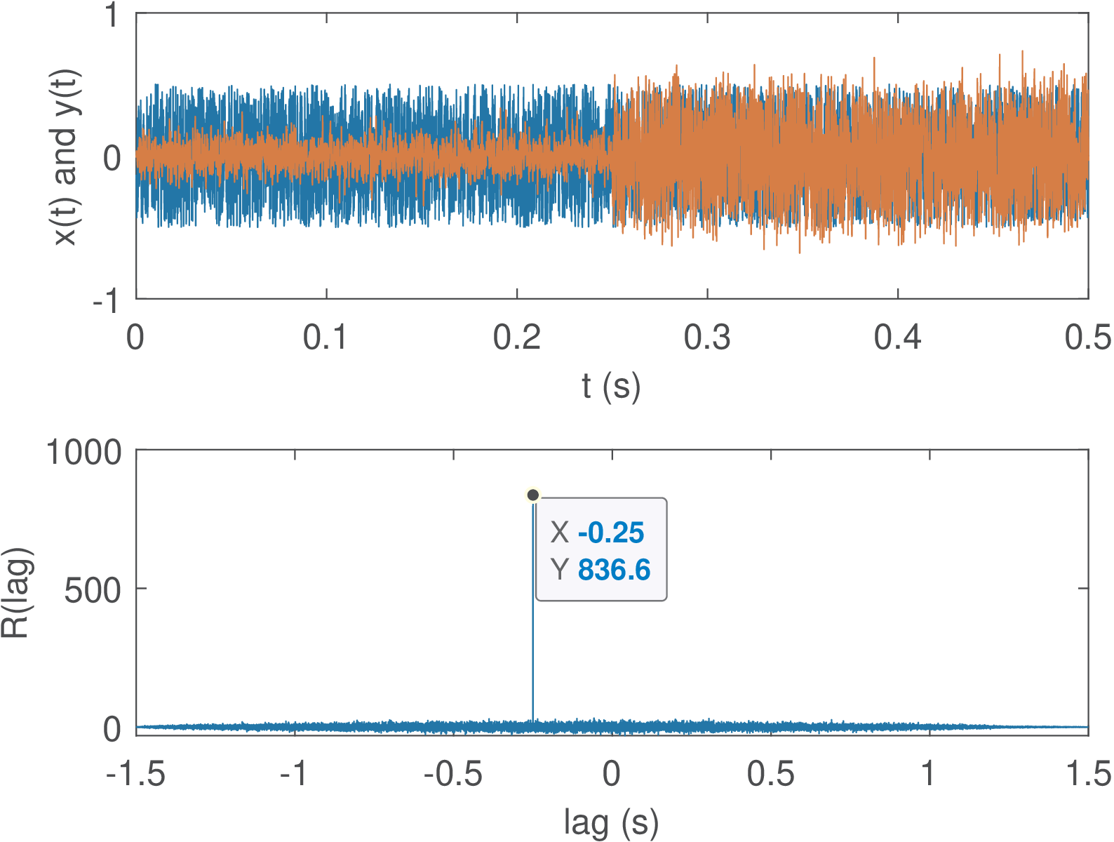
After running the code as it is, observe what happens if x=rand(1,N), i. e., use a signal with a mean different than zero (0.5, in this case). In this case, the correlation is affected in a way that the peak indicating the delay is less pronounced. Another test is to use a cosine (modify the if) with delayInSamples assuming a small value with respect to the total length N of the vectors. The estimation can fail, indicating the delay to be zero. Another parameter to play with is the SNR. Use values smaller than 10 dB to visualize how the correlation can be useful even with negative SNR.

It is important to address another issue: comparing vectors of different length. Assume two signals $x[n]$ and $y[n]$ should be aligned in time and then compared sample-by-sample, for example to calculate the error $x[n]-y[n]$. There is a small problem for Matlab/Octave if the vectors have a different length. Assuming that xcorr(x,y) indicated the best lag is positive ($L>0$), an useful post-processing for comparing $x[n]$ and $y[n]$ is to delete samples of $x[n]$. If $L$ is negative, the first samples of $y[n]$ can be deleted. Listing 1.30 illustrates the operation and makes sure that the vectors representing the signals have the same length.

1x=[1 -2 3 4 5 -1]; %some signal 
2y=[3 1 -2 -2 1 -4 -3 -5 -10]; %the other signal 
3[c,lags]=xcorr(x,y); %find crosscorrelation 
4L = lags(find(abs(c)==max(abs(c)))); %lag for the maximum 
5if L>0 
6  x(1:L)=[]; %delete first L samples from x 
7else 
8  y(1:-L)=[]; %delete first L samples from y 
9end 
10if length(x) > length(y) %make sure lengths are the same 
11  x=x(1:length(y)); 
12else 
13  y=y(1:length(x)); 
14end 
15plot(x-y); title('error between aligned x and y');  

Elaborate and execute the following experiment: record two utterances of the same word, storing the first in a vector x and the second in y. Align the two signals via cross-correlation and calculate the mean-squared error (MSE) between them (for the MSE calculation it may be necessary to have vectors of the same length, as discussed).   $\text{□}$