Analog, Digital and Discrete-Time Signals

1.2 Analog, Digital and Discrete-Time Signals

In general, a signal is anything that can be transmitted or stored, and represents useful information.

Few examples can illustrate what information means in this context. For example, monochromatic and color images are two-dimensional (2D) and 3D signals, respectively, in which the information are the pixel values. For instance, a color image $X$ with resolution of $480 \times 640$ pixels can be represented in the RGB color space¹ by a 3D matrix with dimension $480 \times 640 \times 3$ .

A video is a sequence $X [n]$ of images (each one called a frame) that are indexed by the integer $n$ . While an image $X$ does not depend on time, the value of $n$ in the video $X [n]$ is interpreted as the time instant. For example, a video $X [n]$ with 500 frames can be represented by a 4D multidimensional array (also called tensor) of dimension $500 \times 480 \times 640 \times 3$ , in which $X = X [3]$ is the image (frame) with dimension $480 \times 640 \times 3$ corresponding to time $n = 3$ .

Another example of a signal is the electrocardiogram (ECG). Typically, the ECG is recorded with several channels and constitutes a multivariate or multidimensional signal $x (t)$ , where $t$ is the time dimension. The information in the ECG corresponds to the amplitudes of each channel, which for a given $t$ can be organized as a vector $x$ . For instance, assuming six channels and a given time $t_{0}$ , the vector $x = x (t_{0})$ contains the six amplitude values.

The provided examples illustrate that there are signals with very different characteristics. To simplify the initial discussion, unless otherwise stated, it is assumed hereafter a one-dimensional real-valued signal that describes how a single amplitude varies over time.

It is useful to classify signals according to the behavior of these two variables: the independent variable representing progress in time and the amplitude, which is the dependent variable. If time evolution is represented by a real-valued variable $t \in ℝ$ , the function $x (t)$ is called a continuous-time signal. If the progress over time is represented by an integer index $n \in ℤ$ , the sequence $x [n]$ is called a discrete-time signal.

Similarly, the amplitude can freely assume any real value or be restricted to only pre-specified values from a finite set $ℳ$ . In the latter case, the amplitude is said to be quantized. The quantized amplitudes can be eventually non-integer numbers. The number $M$ of elements in $ℳ$ , i. e., the cardinality $M = | ℳ |$ , indicates whether the system is binary ( $M = 2$ ), quaternary ( $M = 4$ ) or $M$ -ary. A subscript $q$ will be used to denote a quantized signal, such as in $x_{q} (t)$ .

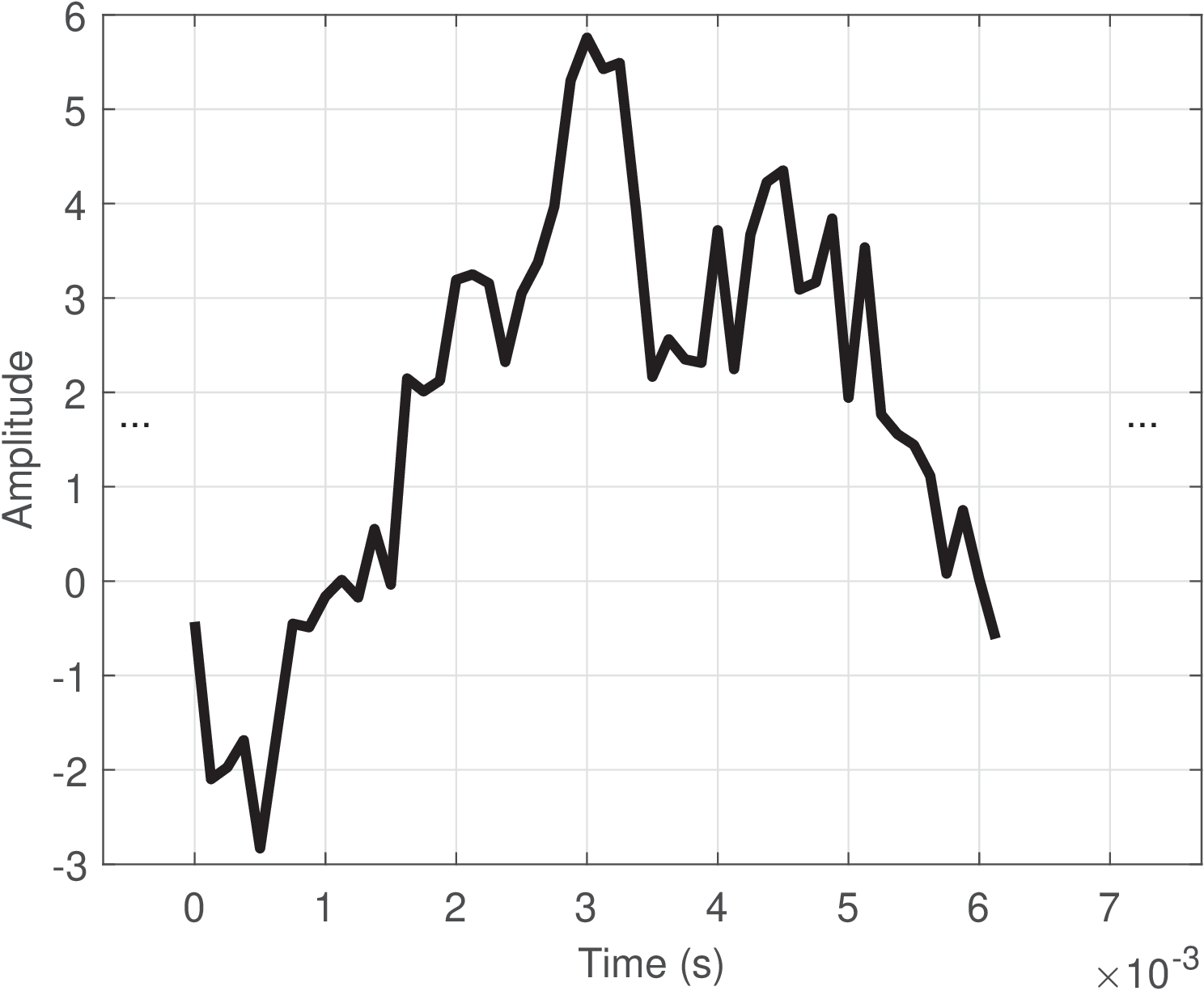
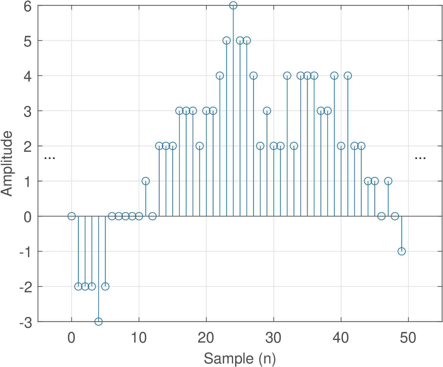
Based on the previous definitions, it is possible to define analog and digital signals, which are the most common signals in practice. A digital signal $x_{q} [n]$ is a discrete-time signal with quantized amplitudes. An analog signal $x (t)$ is a continuous-time signal in which the amplitudes are not quantized (are not restricted to a finite number of $M$ distinct values). Table 1.1 summarizes a useful taxonomy of signals. Figure 1.1 and Figure 1.2 provide examples of analog and digital signals, respectively.

Table 1.1: Notation used for continuous and discrete-time signals.

	Continuous-time, $t \in ℝ$	Discrete-time, $n \in ℤ$
Quantized amplitude	$x_{q} (t)$	$x_{q} [n]$ (digital)
Not quantized	$x (t)$ (analog)	$x [n]$

Figure 1.1: Example of analog signal. Note the abscissa is continuous and the amplitude is not quantized, assuming an infinite number of possible values.

Figure 1.2: Example of digital signal obtained by digitalizing the analog signal in Figure 1.1. Note both the abscissa (dimensionless indices) and amplitude of the digital signal are discrete. In this case, the quantized amplitudes assume $M = 10$ possible values from $ℳ = {- 3, - 2, \dots, 5, 6}$ .

Signals that exist in the real-world are inherently analog. Even a DC power supply regulated to output 0 or 5 volts will present a small random amplitude fluctuation due to circuit imperfections and noise. It could then be (strictly) classified as an analog signal $x (t)$ . But the circuits of a traditional digital system (e. g., a computer) can tolerate amplitude variations within a given range and, consequently, one may want to model such signal as continuous in time and with quantized amplitudes, denoting it as $x_{q} (t)$ . It is also possible to find authors calling such continuous-time signal with quantized amplitudes $x_{q} (t)$ a “digital” signal, but this nomenclature will be avoided in this text.

The interfaces between digital systems and the analog world require analog to digital (A/D) and digital to analog (D/A) conversions, which will be discussed in Section 1.7.

1.2.1 Advanced: Ambiguous notation: whole signal or single sample

It should be noted that the notation $x [n]$ (the same happens for $x (t)$ ) is ambiguous in the sense that it is widely used to represent both: a) the complete sequence and b) a sample at time $n$ . In most scenarios both interpretations are valid because if someone provides an equation such as

x [n] = 3 n,

(1.1)

which is valid for all $n \in ℤ$ , this equation can be repeatedly used to reconstruct the whole sequence by varying $n$ , or be interpreted as a single sample for a specific value $n = n_{0}$ . In some cases, to disambiguate the two interpretations, a notation such as $x [n_{0}]$ or $x (t_{0})$ is adopted, where $n_{0}$ and $t_{0}$ denote specific time instants instead of a generic variable that can be iteratively used to represent the complete sequence.²

1.2.2 Digitizing signals

In many digital signal processing applications, it is required to convert a real-world analog signal into a digital format, and then process it with a computer, microcontroller, FPGA (field programmable gate array) or digital signal processor (DSP) chip, for example. Therefore, a brief review of the A/D process is discussed in the sequel.

The A/D converter (or ADC chip) transforms the input analog signal $x (t)$ into a digital signal $x_{q} [n]$ , consisting of a sequence of quantized samples. The ADC executes two tasks:

sampling: periodically extract samples to accurately describe the signal;
quantization: represent each of these samples with a reasonable accuracy.

Sampling depends on the adopted sampling frequency $F_{s}$ , which is the number of samples extracted from the signal per time unit (more specifically, one second).³ For example, $F_{s} = 8000$ Hz corresponds to obtaining 8000 samples to represent each signal segment with a duration of 1 second. The higher $F_{s}$ , the more accurate the representation tends to be.

Quantization depends on the number $b$ of bits used to represent each sample. For example, if $b = 2$ , each sample can be represented by only $N = 4$ distinct values: 00, 01, 10 and 11. The mapping between these binary values and amplitudes is somehow arbitrary. For example, 00 can represent $- 10$ V while 01 can represent $- 5$ V. In general, an ADC of $b$ bits can output $N = 2^{b}$ distinct quantized values.

ADCs with large values for $F_{s}$ and $b$ are more expensive. Sometimes the tradeoff is to use a relatively large $F_{s}$ with small $b$ (e.g., $F_{s} = 2.2$ GHz with $b = 10$ bits) or vice-versa (e.g., $F_{s} = 2.5$ MHz with $b = 24$ bits).

The chip that performs the digital to analog conversion is called DAC. It also operates according to the values of $F_{s}$ and $b$ .

Note that the operation performed by an ADC chip is in general lossy and, consequently, non-invertible.⁴ Therefore, cascading an ADC and a DAC chips recovers only an approximation of the original signal $x (t)$ . In this text we will learn how to properly choose $F_{s}$ and $b$ to control the A/D and D/A processes, in order to recover $x (t)$ with the accuracy that the given application demands. These two parameters are the most relevant in the A/D and D/A processes, but when choosing commercial chips, there are many others (see exercises in Section 1.16) . One important figure of merit to estimate this accuracy is the signal-to-noise ratio (SNR), which is the ratio between the power of the input $x (t)$ and the power of the “noise” signal, which in this case is the total error caused by the sampling and quantization processing stages. When this error is solely caused by quantization, the SNR is called signal-to-quantization-noise ratio (SQNR).

1.2.3 Discrete-time signals

In practice, the A/D conversion is typically performed by a monolithic ADC chip. But for theoretical studies, it is convenient to mathematically model this A/D conversion by splitting it in the two mentioned stages: sampling and quantization. One important reason for adopting these two stages when modeling the A/D conversion is that, while sampling is a linear operation, the input-output relation of quantizers is nonlinear (you may want to take a peek at Figure 1.53 and note that the relation corresponds to a non-linear stairs function). There are several tools, such as the Laplace and Fourier transforms discussed in Chapter 2 for dealing with linear operations. On the other hand, working with nonlinear systems is more evolved. Because of that, most “digital” signal processing theory does not assume the amplitude is quantized to enable the usage of tools restricted to linear operations. Hence, more strictly, most of the DSP theory could be called “discrete-time” signal processing. However, the name “digital signal processing” is more popular.

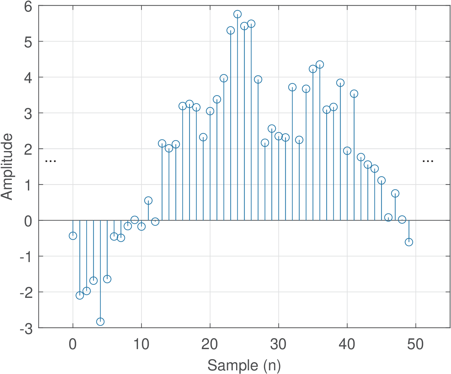
Figure 1.3: Example of discrete-time signal $x [n]$ . Note the abscissa is discrete, but the amplitude (ordinate) is not quantized.

Figure 1.3 illustrates a discrete-time signal. Note the abscissa is given in discrete-time $n \in ℕ$ , similar to the notation adopted for digital signals. But for a discrete-time signal $x [n]$ , the amplitude is not quantized and can assume any value. Figure 1.3 should be compared with Figure 1.1 and Figure 1.2, observing each axis.

Example 1.1. Example of creating a discrete-time signal from a continuous-time sinusoid. Consider extracting samples from the analog signal $x (t) = 6 cos (2 π 400 t)$ with amplitude 6 volts and a frequency $f_{c} = 400$ Hz (the subscript $c$ is just to indicate this is a specific and fixed frequency value). The goal is to use $F_{s} = 8000$ samples to represent each segment of one second, where $F_{s}$ is the sampling frequency. The time interval between consecutive samples is $T_{s} = 1 ∕ F_{s}$ , which in this case is $T_{s} = 1 ∕ 8000 = 125$ $μ$ s. Listing 1.1 illustrates one possible implementation.

Listing 1.1: MatlabOctaveCodeSnippets/snip_signals_signal_generation.m. [ Python version]

1Fs=8000; %sampling frequency (Hz) 
2Ts=1/Fs; %sampling interval (seconds) 
3f0=400; %cosine frequency (Hz) 
4N=100; %number of desired samples 
5n=0:N-1; %generate discrete-time abscissa 
6t=n*Ts; %discretized continuous-time axis (sec.) 
7x=6*cos(2*pi*f0*t); %amplitude=6 V and frequency = f0 Hz 
8stem(n,x); %plot discrete-time signal

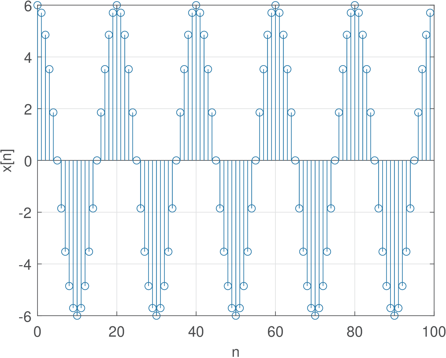
Figure 1.4: Example of a discrete-time cosine generated with Listing 1.1.

Figure 1.4 indicates the result of executing Listing 1.1. This cosine has a period of $T = 1 ∕ f_{c} = 1 ∕ 400 = 2.5$ ms. Therefore, each of its period is being represented by $T ∕ T_{s} = (2.5 \times 1 0^{- 3}) ∕ (125 \times 1 0^{- 6}) = 20$ samples. Note in Figure 1.4 that, in this specific case, at each sample $n = 20, 40, 60, \dots$ , the sample $x [0] = 6$ at $n = 0$ is repeated, and a new cosine cicle starts. $□$

1.2.4 Brief introduction to frequency-domain analysis

In subsequent chapters, the task of representing signals in frequency-domain will be thoroughly discussed. But it is convenient to anticipate a very brief introduction of a key aspect of Fourier analysis: the capability of decomposing a signal into its frequency components. For instance, by inspection, a signal

x (t) = 500 cos (2000 πt + 0.3) + 2 cos (7000 πt + π)

(1.2)

is composed of two frequency components. The first one is a cosine with an amplitude of 500 V, phase of 0.3 radians and angular frequency $ω = 2 πf = 2000 π$ rad/s, which corresponds to a frequency $f = ω ∕ (2 π) = 1000$ Hz. The second frequency component has an amplitude of 2 V, phase of $π$ radians and angular frequency of $ω = 7000 π$ rad/s (corresponding to $f = 3500$ Hz). The Fourier analysis provides exactly this kind of information about the frequency components that, when added together, creates the corresponding time-domain signal.

There are many techniques based on Fourier analysis that represent information about the frequency components of a signal. Few examples are provided below:

Spectrum: informs the frequency, magnitude and phase of each frequency component of the corresponding signal.
PSD: power spectral density (PSD) provides information on how the signal power is distributed over frequency.
Spectrogram: describes how power is distributed over both time and frequency, using a representation that corresponds to calculating several PSDs over different time segments.

The frequency components of the signal in Eq. (1.2) are depicted in Figure 1.5 using two distinct graphs: one for amplitude (top) and another for phase. The plots were obtained using a duration of 14 s for $x (t)$ but information about signal duration is not available from spectrum plots.

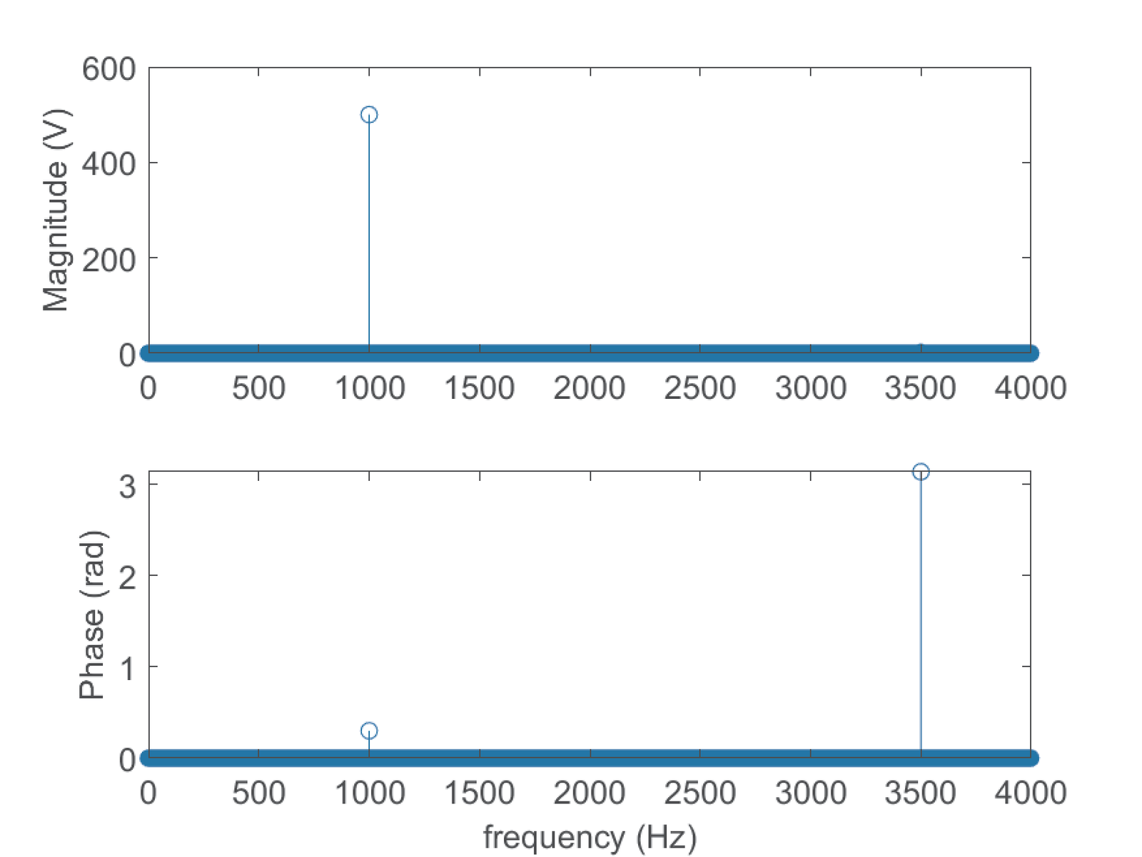
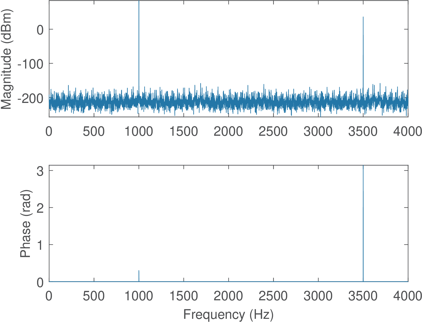
Figure 1.5: Spectrum magnitude in volts (top) and phase in radians (bottom) of the signal composed of two cosines, as indicated in Eq. (1.2). The magnitude of the component at 3500 Hz is relatively small and does not show up.

When compared to 500 V of the first component of $x (t)$ in Eq. (1.2), the magnitude of 2 V of the component at 3500 Hz is relatively small and does not show up when the magnitude is depicted in linear scale in Figure 1.5. Alternatively, Figure 1.6 represents the magnitude in dBm and make evident the two frequency components. Another distinction is that Figure 1.6 uses Matlab’s plot method, while Figure 1.5 uses Matlab’s stem method.

Figure 1.6: Spectrum magnitude in dBm (top) and phase in radians (bottom) of the signal composed of two cosines, as indicated in Eq. (1.2).

When it is not required to obtain information about the phase of the frequency components, it may be convenient to represent the frequency components using the PSD or the spectrogram. Figure 1.7 provides an example using the same signal of Eq. (1.2). In this case, the duration of 14 s can be observed from the spectrogram.

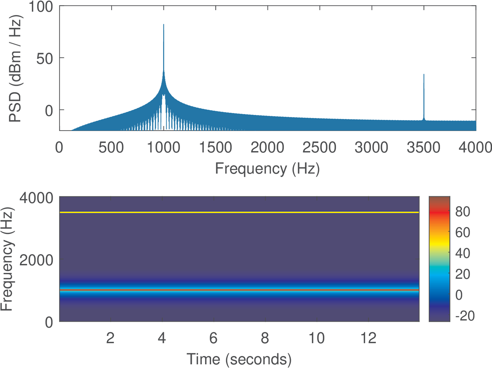
Figure 1.7: PSD (top) and spectrogram (bottom) of the signal composed of two cosines, as indicated in Eq. (1.2).

It can be seen from Figure 1.7 that the spectrogram is a redundant representation when the magnitudes of the frequency components do not change over time. To compare with Figure 1.7, it is pedagogical to consider the spectrogram of a new signal $z (t)$ , which has the same duration of 14 s, and is composed of the frequency component $500 cos (2000 πt + 0.3)$ along half of the time duration (7 s) and $2 cos (7000 πt + π)$ during the second half. First, Figure 1.8 shows the spectrum of the new signal $z (t)$ .

Figure 1.8: Magnitude spectrum (dBm) and phase spectrum (rad) of a signal formed by concatenating two cosine waveforms with different frequencies, amplitudes, and phases.

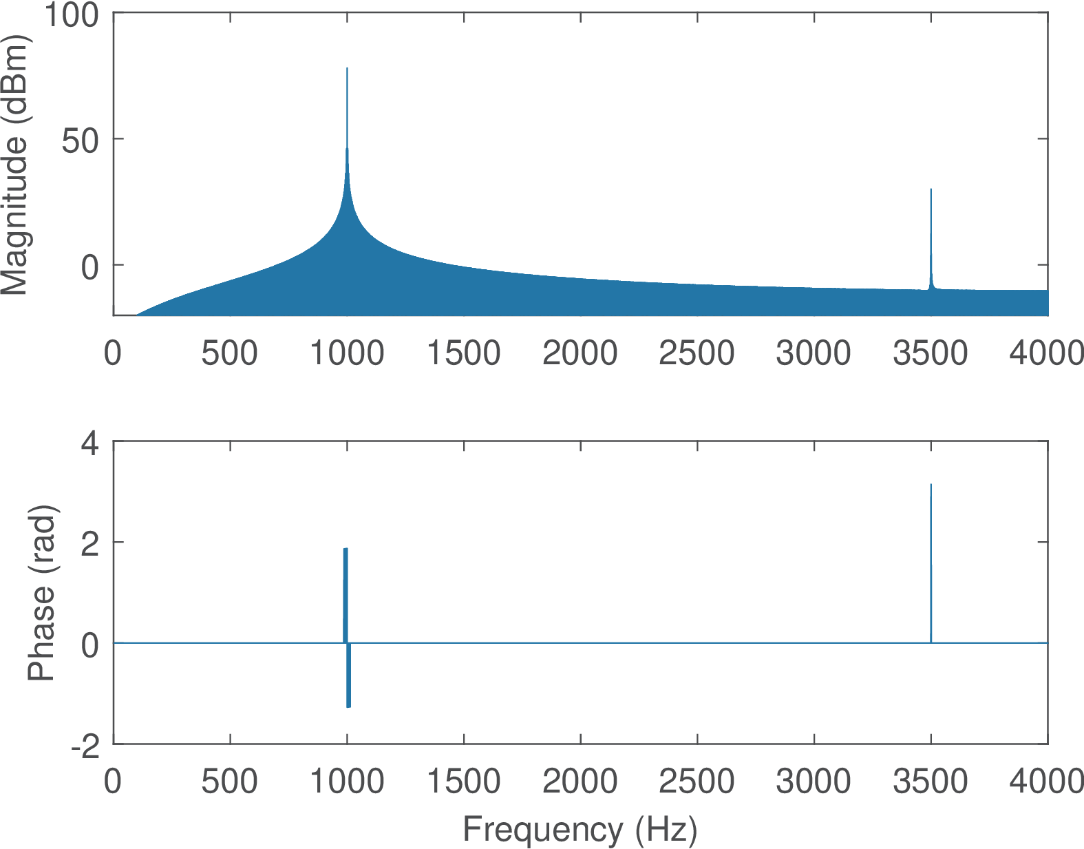
Comparing Figure 1.8 and Figure 1.6 one can notice that the two spectra are similar. The concatenation process affected primarily the phase of $z (t)$ , which differs from the phases of the components of $x (t)$ . Figure 1.9 depicts the PSD and spectrogram of $z (t)$ .

Figure 1.9: PSD (top) and spectrogram (bottom) of a signal formed by concatenating two cosine waveforms with different frequencies, amplitudes, and phases.

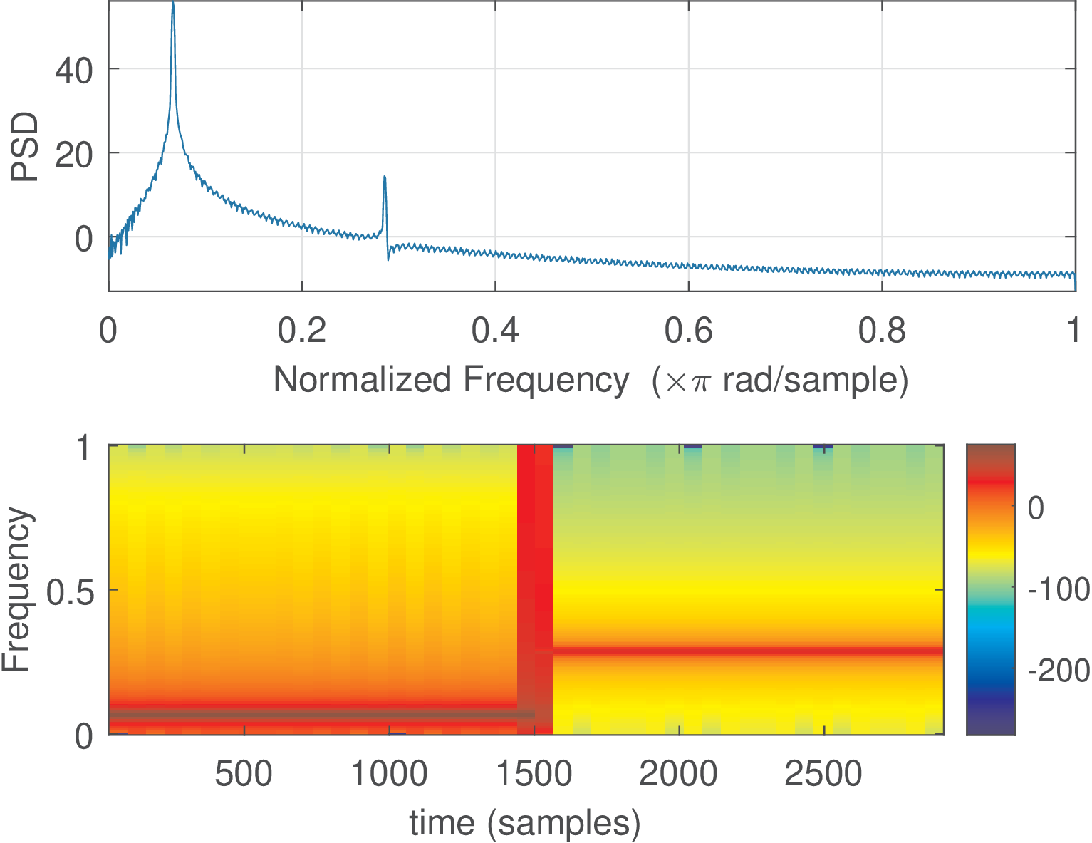
The spectrograms in Figure 1.7 and Figure 1.9 indicate how the magnitude of the frequency components of $x (t)$ and $z (t)$ , respectively, change over time. For instance, Figure 1.9 successfully performs the job of indicating that around $t = 7$ s an abrupt change occurred and $z (t)$ starts to have a higher frequency (3500 Hz) with a lower amplitude (indicated by the colorbar). In contrast, the spectrum and PSD plots are capable of describing the existence of two frequency components but are unable of informing their location in time.

The spectrogram generates a representation in both time and frequency domains because it extracts segments from the input signal (e. g. $x (t)$ ) and calculates the spectrum of each of these several segments (also called windows). The spectrogram is stored as a matrix in which an element corresponds to a specific point in the time $\times$ frequency grid, and stores the magnitude of the spectrum. A sliding window is used to obtain distinct (eventually overlapping) segments, and the input parameters window shift and window length define the amount of time (or, equivalently, the number of samples of a discrete-time signal) the window is moved at each segment extraction and its total duration.

For future similar analysis, the Matlab/Octave functions ak_spectrum, ak_psd and ak_specgram can be used to estimate the spectrum, PSD and spectrogram of discrete-time signals.⁵

For example, Listing 1.2 was used to generate $z (t)$ and later obtaining Figure 1.8 and Figure 1.9.

Listing 1.2: MatlabOctaveCodeSnippets/snip_frequency_cosine_spectogram.m

1Fs=8000; %sampling frequency (Hz) 
2Ts=1/Fs; %sampling interval (seconds) 
3N=Fs * 14; %number of samples assuming a signal duration of 14 secs 
4n=0:N-1; %generate discrete-time abscissa 
5t=n*Ts; %discretized continuous-time axis (sec.) 
6t0=t(1:N/2); %first time segment 
7t1=t(N/2+1:end); %second time segment 
8f0=1000; %cosine frequency (Hz) 
9x0=500*cos(2*pi*f0*t0+0.3); %signal segment for first half 
10f1=3500; %cosine frequency (Hz) 
11x1=2*cos(2*pi*f1*t1+pi); %signal segment for first half 
12z=[x0 x1]; %concatenation of 2 cosines 
13[Z,f] = ak_spectrum(z, Fs); %spectrum for real-valued signals 
14subplot(211) 
15plot(f,20*log10(abs(Z)) + 30); %add 30 to convert dBW into dBm 
16ylabel('Magnitude (dBm)'), axis([0, Fs/2, -20, 100]) 
17subplot(212) 
18plot(f,angle(Z)); 
19xlabel('Frequency (Hz)'); ylabel('Phase (rad)')

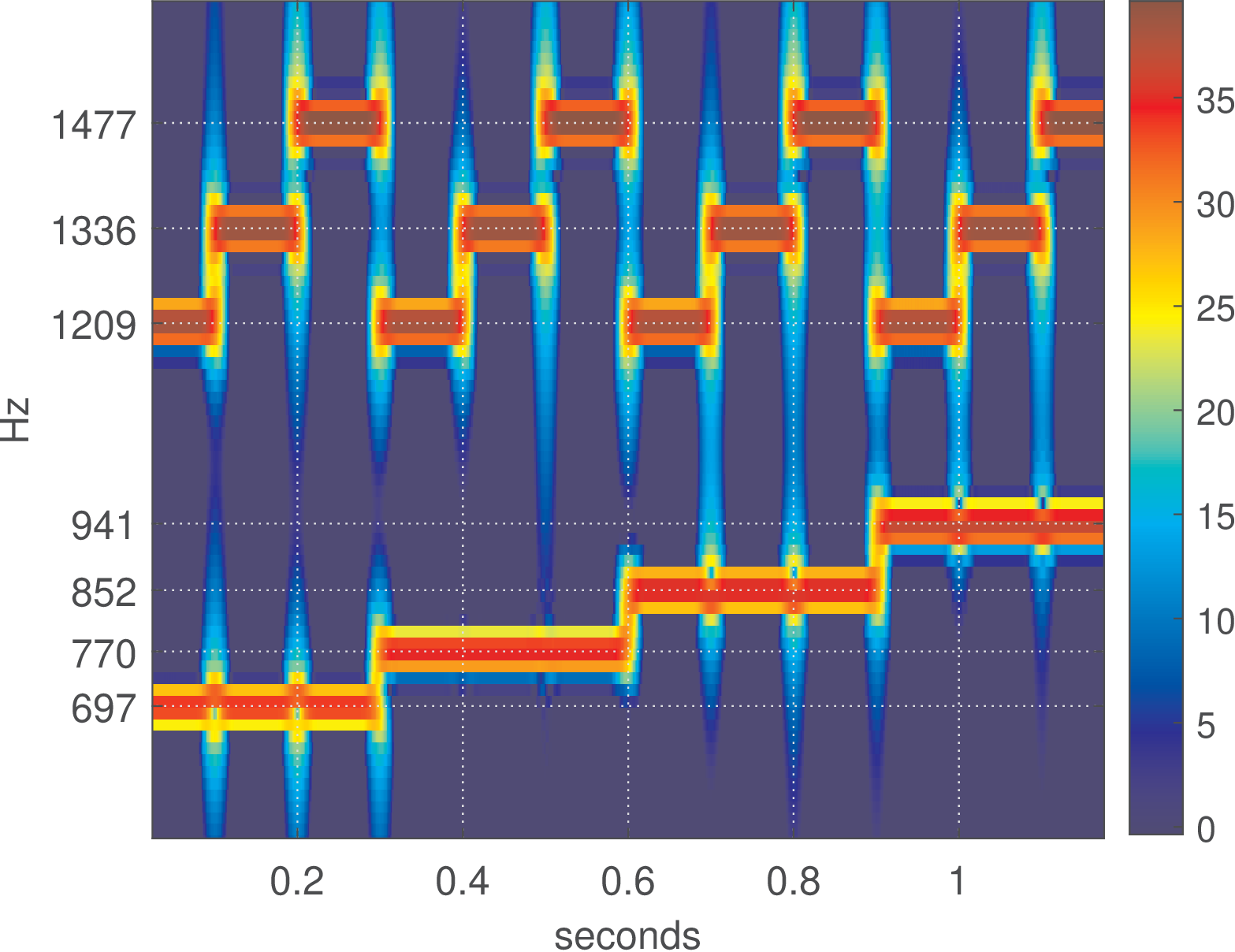
Figure 1.10: All twelve DTMF symbols: 1-9,*,0,#, each one composed by a sum of a low [697,770,852,941] and a high [1209,1336,1477] (Hz) frequencies.

As another example of how spectrograms are useful, Figure 1.10 shows a sequence of all twelve dual-tone multi-frequency (DTMF) tones generated by the script figs_spectral_dtmf.m. In this case, each symbol has a 100 ms duration. It is possible to visually decode the signal. For example, the first symbol (left-most) is composed by a sum of sines of frequencies 697 and $1, 209$ Hz (representing “1”) while the second is composed by frequencies 697 and $1, 336$ Hz (symbol “2”) and so on.

After creating dtmfSignal with $F_{s} = 8$ kHz, the spectrogram of Figure 1.10 was generated with the commands below, and for a better visualization, the dynamic range was restricted to 40 dB via the parameter thresholdIndB:

1filterBWInHz=40; %equivalent FFT bandwidth in Hz 
2samplingFrequency=8000; %sampling frequency in Hz 
3windowShiftInms=1; %window shift in miliseconds 
4thresholdIndB=40; %discards low power values below it 
5ak_specgram(dtmfSignal,filterBWInHz,samplingFrequency,... 
6   windowShiftInms,thresholdIndB) %calculate spectrogram

¹ RGB stands for the colors red, green and blue.

² This notation will be adopted, for instance, in Eq. (1.4).

³ Some authors prefer to reserve the unit Hertz (Hz) to only represent the oscillation rate of signals, electrical fields, etc., sticking with its historical use. With this motivation, they avoid, for example, to denote the sampling frequency $F_{s}$ of an ADC in Hz and use samples per second (SPS) instead. In this text, Hz is “overloaded” to be a unit that can account for everything repeating a given number of times per second and $F_{s}$ is reported in Hz.

⁴ A lossless operation from $x$ to $y$ , allows recovering $\hat{x}$ from $y$ , such that $\hat{x} = x$ . If the operation is lossy, then $\hat{x} = x + e$ , where $e$ is a non-zero error.

⁵ Matlab (but not Octave) has the spectrogram function. The specgram function was discontinued in Matlab.